

Wind-driven circulation
109
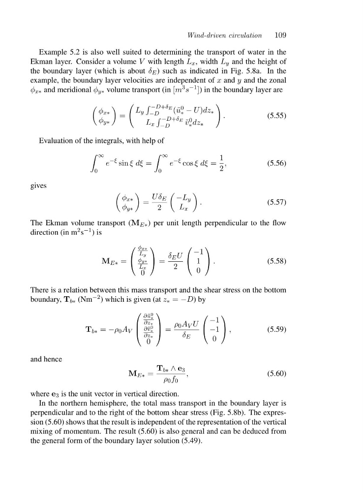
Example 5.2 is also well suited to determining the transport of water in the
Ekman layer. Consider a volume V with length L x , width L y and the height of
the boundary layer (which is about δ E ) such as indicated in Fig. 5.8a. In the
example, the boundary layer velocities are independent of x and y and the zonal
φ x∗ and meridional φ y∗ volume transport (in [m 3 s −1 ]) in the boundary layer are
φ x∗
φ y∗
=
L y
−D+δ E
−D
(˜ u 0
∗ − U )dz ∗
L x
−D+δ E
−D
˜
v 0
∗ dz ∗
.
(5.55)
Evaluation of the integrals, with help of
∞
0
e
−ξ sin ξdξ=
∞
0
e
−ξ cos ξdξ=
1
2
,
(5.56)
gives
φ x∗
φ y∗
=
Uδ E
2
−L y
L x
.
(5.57)
The Ekman volume transport (M E∗ ) per unit length perpendicular to the flow
direction (in m 2 s −1 )is
M E∗ =
⎛
⎝
φx∗
Ly
φy∗
Lx
0
⎞
⎠ =
δ E U
2
⎛
⎝
−1
1
0
⎞
⎠ .
(5.58)
There is a relation between this mass transport and the shear stress on the bottom
boundary, T b∗ (Nm −2 ) which is given (at z ∗ = −D)by
T b∗ = −ρ 0 A V
⎛
⎜
⎝
∂ ˜
u 0
∗
∂z∗
∂˜ v 0
∗
∂z∗
0
⎞
⎟
⎠ =
ρ 0 A V U
δ E
⎛
⎝
−1
−1
0
⎞
⎠ ,
(5.59)
and hence
M E∗ =
T b∗ ∧ e 3
ρ 0 f 0
,
(5.60)
where e 3 is the unit vector in vertical direction.
In the northern hemisphere, the total mass transport in the boundary layer is
perpendicular and to the right of the bottom shear stress (Fig. 5.8b). The expression (5.60) shows that the result is independent of the representation of the vertical
mixing of momentum. The result (5.60) is also general and can be deduced from
the general form of the boundary layer solution (5.49).
109
Example 5.2 is also well suited to determining the transport of water in the
Ekman layer. Consider a volume V with length L x , width L y and the height of
the boundary layer (which is about δ E ) such as indicated in Fig. 5.8a. In the
example, the boundary layer velocities are independent of x and y and the zonal
φ x∗ and meridional φ y∗ volume transport (in [m 3 s −1 ]) in the boundary layer are
φ x∗
φ y∗
=
L y
−D+δ E
−D
(˜ u 0
∗ − U )dz ∗
L x
−D+δ E
−D
˜
v 0
∗ dz ∗
.
(5.55)
Evaluation of the integrals, with help of
∞
0
e
−ξ sin ξdξ=
∞
0
e
−ξ cos ξdξ=
1
2
,
(5.56)
gives
φ x∗
φ y∗
=
Uδ E
2
−L y
L x
.
(5.57)
The Ekman volume transport (M E∗ ) per unit length perpendicular to the flow
direction (in m 2 s −1 )is
M E∗ =
⎛
⎝
φx∗
Ly
φy∗
Lx
0
⎞
⎠ =
δ E U
2
⎛
⎝
−1
1
0
⎞
⎠ .
(5.58)
There is a relation between this mass transport and the shear stress on the bottom
boundary, T b∗ (Nm −2 ) which is given (at z ∗ = −D)by
T b∗ = −ρ 0 A V
⎛
⎜
⎝
∂ ˜
u 0
∗
∂z∗
∂˜ v 0
∗
∂z∗
0
⎞
⎟
⎠ =
ρ 0 A V U
δ E
⎛
⎝
−1
−1
0
⎞
⎠ ,
(5.59)
and hence
M E∗ =
T b∗ ∧ e 3
ρ 0 f 0
,
(5.60)
where e 3 is the unit vector in vertical direction.
In the northern hemisphere, the total mass transport in the boundary layer is
perpendicular and to the right of the bottom shear stress (Fig. 5.8b). The expression (5.60) shows that the result is independent of the representation of the vertical
mixing of momentum. The result (5.60) is also general and can be deduced from
the general form of the boundary layer solution (5.49).