

108
DYNAMICAL OCEANOGRAPHY
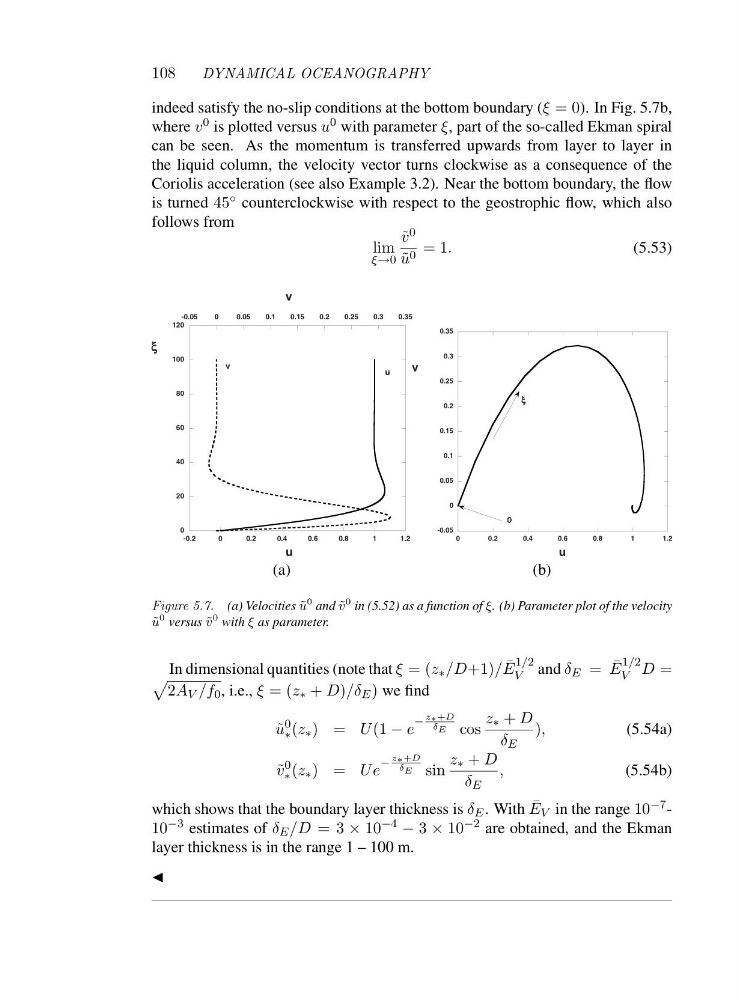
indeed satisfy the no-slip conditions at the bottom boundary (ξ =0). In Fig. 5.7b,
where v 0 is plotted versus u 0 with parameter ξ, part of the so-called Ekman spiral
can be seen. As the momentum is transferred upwards from layer to layer in
the liquid column, the velocity vector turns clockwise as a consequence of the
Coriolis acceleration (see also Example 3.2). Near the bottom boundary, the flow
is turned 45 ◦ counterclockwise with respect to the geostrophic flow, which also
follows from
lim
ξ→0
˜
v 0
˜
u 0 =1.
(5.53)
0
20
40
60
80
100
120
-0.2
0
0.2
0.4
0.6
0.8
1
1.2
-0.05
0
0.05
0.1
0.15
0.2
0.25
0.3
0.35
v
u
ξ ξ ξ
ξ
v
u
(a)
-0.05
0
0.05
0.1
0.15
0.2
0.25
0.3
0.35
0
0.2
0.4
0.6
0.8
1
1.2
u
v
0 0
0
0
ξ ξ ξ
ξ
(b)
Figure 5.7. (a) Velocities ˜
u
0 and ˜
v
0 in (5.52) as a function of ξ. (b) Parameter plot of the velocity
˜
u
0 versus ˜
v
0 with ξ as parameter.
In dimensional quantities (note that ξ =(z ∗ /D+1)/ ¯
E
1/2
V and δ E = ¯
E
1/2
V D =
2A V /f 0 , i.e., ξ =(z ∗ + D)/δ E ) we find
˜
u
0
∗ (z ∗ )=U (1 − e
−
z∗+D
δ E
cos
z ∗ + D
δ E
),
(5.54a)
˜
v
0
∗ (z ∗ )=Ue
−
z∗+D
δ E
sin
z ∗ + D
δ E
,
(5.54b)
which shows that the boundary layer thickness is δ E . With ¯
E V in the range 10 −7 -
10 −3 estimates of δ E /D =3× 10 −4 − 3 × 10 −2 are obtained, and the Ekman
layer thickness is in the range 1 – 100 m.
◭
DYNAMICAL OCEANOGRAPHY
indeed satisfy the no-slip conditions at the bottom boundary (ξ =0). In Fig. 5.7b,
where v 0 is plotted versus u 0 with parameter ξ, part of the so-called Ekman spiral
can be seen. As the momentum is transferred upwards from layer to layer in
the liquid column, the velocity vector turns clockwise as a consequence of the
Coriolis acceleration (see also Example 3.2). Near the bottom boundary, the flow
is turned 45 ◦ counterclockwise with respect to the geostrophic flow, which also
follows from
lim
ξ→0
˜
v 0
˜
u 0 =1.
(5.53)
0
20
40
60
80
100
120
-0.2
0
0.2
0.4
0.6
0.8
1
1.2
-0.05
0
0.05
0.1
0.15
0.2
0.25
0.3
0.35
v
u
ξ ξ ξ
ξ
v
u
(a)
-0.05
0
0.05
0.1
0.15
0.2
0.25
0.3
0.35
0
0.2
0.4
0.6
0.8
1
1.2
u
v
0 0
0
0
ξ ξ ξ
ξ
(b)
Figure 5.7. (a) Velocities ˜
u
0 and ˜
v
0 in (5.52) as a function of ξ. (b) Parameter plot of the velocity
˜
u
0 versus ˜
v
0 with ξ as parameter.
In dimensional quantities (note that ξ =(z ∗ /D+1)/ ¯
E
1/2
V and δ E = ¯
E
1/2
V D =
2A V /f 0 , i.e., ξ =(z ∗ + D)/δ E ) we find
˜
u
0
∗ (z ∗ )=U (1 − e
−
z∗+D
δ E
cos
z ∗ + D
δ E
),
(5.54a)
˜
v
0
∗ (z ∗ )=Ue
−
z∗+D
δ E
sin
z ∗ + D
δ E
,
(5.54b)
which shows that the boundary layer thickness is δ E . With ¯
E V in the range 10 −7 -
10 −3 estimates of δ E /D =3× 10 −4 − 3 × 10 −2 are obtained, and the Ekman
layer thickness is in the range 1 – 100 m.
◭