

Wind-driven circulation
107
pressure gradient, which is independent of the vertical coordinate since throughout
the water column ˜
p 0 (x, y)=p 0 (x, y). The matching principle for the pressure
takes a simple form here.
The boundary layer (inner) solution becomes
˜
u
0 (x, y, ξ)=u
0 (x, y)(1 − e
−ξ cos ξ) − v
0 (x, y)e
−ξ sin ξ, (5.49a)
˜
v
0 (x, y, ξ)=v
0 (x, y)(1 − e
−ξ cos ξ)+u
0 (x, y)e
−ξ sin ξ, (5.49b)
and from (5.44d) we find for ˜
w 0
˜
w
0 (x, y, ξ)=
ζ 0
2
(1 − e
−ξ (cos ξ +sinξ)),
(5.50)
where ζ 0 is the vertical component of the O(1) vorticity defined by
ζ
0 =
∂v 0
∂x
−
∂u 0
∂y
.
(5.51)
◮
Example 5.2: Ekman bottom layer solution
δ E
f 0
Ekman boundary layer
Geostrophic flow
U
g
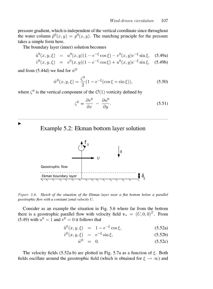
Figure 5.6. Sketch of the situation of the Ekman layer near a flat bottom below a parallel
geostrophic flow with a constant zonal velocity U .
Consider as an example the situation in Fig. 5.6 where far from the bottom
there is a geostrophic parallel flow with velocity field v ∗ =( U, 0, 0) T .F r o m
(5.49) with u 0 =1and v 0 =0it follows that
˜
u
0 (x, y, ξ)=1 − e
−ξ cos ξ,
(5.52a)
˜
v
0 (x, y, ξ)=e
−ξ sin ξ,
(5.52b)
˜
w
0 =0 .
(5.52c)
The velocity fields (5.52a-b) are plotted in Fig. 5.7a as a function of ξ.B o t h
fields oscillate around the geostrophic field (which is obtained for ξ →∞ )a n d
107
pressure gradient, which is independent of the vertical coordinate since throughout
the water column ˜
p 0 (x, y)=p 0 (x, y). The matching principle for the pressure
takes a simple form here.
The boundary layer (inner) solution becomes
˜
u
0 (x, y, ξ)=u
0 (x, y)(1 − e
−ξ cos ξ) − v
0 (x, y)e
−ξ sin ξ, (5.49a)
˜
v
0 (x, y, ξ)=v
0 (x, y)(1 − e
−ξ cos ξ)+u
0 (x, y)e
−ξ sin ξ, (5.49b)
and from (5.44d) we find for ˜
w 0
˜
w
0 (x, y, ξ)=
ζ 0
2
(1 − e
−ξ (cos ξ +sinξ)),
(5.50)
where ζ 0 is the vertical component of the O(1) vorticity defined by
ζ
0 =
∂v 0
∂x
−
∂u 0
∂y
.
(5.51)
◮
Example 5.2: Ekman bottom layer solution
δ E
f 0
Ekman boundary layer
Geostrophic flow
U
g
Figure 5.6. Sketch of the situation of the Ekman layer near a flat bottom below a parallel
geostrophic flow with a constant zonal velocity U .
Consider as an example the situation in Fig. 5.6 where far from the bottom
there is a geostrophic parallel flow with velocity field v ∗ =( U, 0, 0) T .F r o m
(5.49) with u 0 =1and v 0 =0it follows that
˜
u
0 (x, y, ξ)=1 − e
−ξ cos ξ,
(5.52a)
˜
v
0 (x, y, ξ)=e
−ξ sin ξ,
(5.52b)
˜
w
0 =0 .
(5.52c)
The velocity fields (5.52a-b) are plotted in Fig. 5.7a as a function of ξ.B o t h
fields oscillate around the geostrophic field (which is obtained for ξ →∞ )a n d