

Wind-driven circulation
111
ˆ
ατ
y = −
∂ˆ v 0
∂χ
¯
E
−1/2
V
,
(5.64b)
where τ x and τ y are given functions of x and y. The final solution is
ˆ
u
0 (x, y, χ) − u
0 (x, y)=
αe −χ
2
([τ
y − τ
x ]sinχ +( τ
y + τ
x )cosχ),
(5.65a)
ˆ
v
0 (x, y, χ) − v
0 (x, y)=
αe −χ
2
([τ
y − τ
x ]cosχ − (τ
y + τ
x )sinχ),
(5.65b)
where α =ˆ α ¯
E
1/2
V =2τ 0 /(ρ 0 f 0 δ E U ).
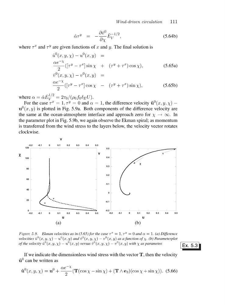
For the case τ x =1 ,τ y =0and α =1 , the difference velocity ˆ
u 0 (x, y, χ) −
u 0 (x, y) is plotted in Fig. 5.9a. Both components of the difference velocity are
the same at the ocean-atmosphere interface and approach zero for χ →∞ .I n
the parameter plot in Fig. 5.9b, we again observe the Ekman spiral; as momentum
is transferred from the wind stress to the layers below, the velocity vector rotates
clockwise.
0
20
40
60
80
100
120
-0.2
-0.1
0
0.1
0.2
0.3
0.4
0.5
-0.2
-0.1
0
0.1
0.2
0.3
0.4
0.5
v
u
χ χ
χ
χ
v
u
(a)
-0.2
-0.1
0
0.1
0.2
0.3
0.4
0.5
-0.2
-0.1
0
0.1
0.2
0.3
0.4
0.5
u
v
χ χ
χ
χ
0 0
0
0
(b)
Figure 5.9. Ekman velocities as in (5.65) for the case τ
x =1,τ
y =0and α =1. (a) Difference
velocities ˆ
u
0 (x, y, χ) − u
0 (x, y) and ˆ
v
0 (x, y, χ) − v
0 (x, y) as a function of χ. (b) Parameterplot
of the velocity ˆ
u
0 (x, y, χ) − u
0 (x, y) versus ˆ
v
0 (x, y, χ) − v
0 (x, y) with χ as parameter.
Ex. 5.3
If we indicate the dimensionless wind stress with the vector T, then the velocity
ˆ
u 0 can be written as
ˆ
u
0 (x, y, χ)=u
0 +
αe −χ
2
(T(cos χ − sin χ)+(T ∧ e 3 )(cos χ +sinχ)). (5.66)
111
ˆ
ατ
y = −
∂ˆ v 0
∂χ
¯
E
−1/2
V
,
(5.64b)
where τ x and τ y are given functions of x and y. The final solution is
ˆ
u
0 (x, y, χ) − u
0 (x, y)=
αe −χ
2
([τ
y − τ
x ]sinχ +( τ
y + τ
x )cosχ),
(5.65a)
ˆ
v
0 (x, y, χ) − v
0 (x, y)=
αe −χ
2
([τ
y − τ
x ]cosχ − (τ
y + τ
x )sinχ),
(5.65b)
where α =ˆ α ¯
E
1/2
V =2τ 0 /(ρ 0 f 0 δ E U ).
For the case τ x =1 ,τ y =0and α =1 , the difference velocity ˆ
u 0 (x, y, χ) −
u 0 (x, y) is plotted in Fig. 5.9a. Both components of the difference velocity are
the same at the ocean-atmosphere interface and approach zero for χ →∞ .I n
the parameter plot in Fig. 5.9b, we again observe the Ekman spiral; as momentum
is transferred from the wind stress to the layers below, the velocity vector rotates
clockwise.
0
20
40
60
80
100
120
-0.2
-0.1
0
0.1
0.2
0.3
0.4
0.5
-0.2
-0.1
0
0.1
0.2
0.3
0.4
0.5
v
u
χ χ
χ
χ
v
u
(a)
-0.2
-0.1
0
0.1
0.2
0.3
0.4
0.5
-0.2
-0.1
0
0.1
0.2
0.3
0.4
0.5
u
v
χ χ
χ
χ
0 0
0
0
(b)
Figure 5.9. Ekman velocities as in (5.65) for the case τ
x =1,τ
y =0and α =1. (a) Difference
velocities ˆ
u
0 (x, y, χ) − u
0 (x, y) and ˆ
v
0 (x, y, χ) − v
0 (x, y) as a function of χ. (b) Parameterplot
of the velocity ˆ
u
0 (x, y, χ) − u
0 (x, y) versus ˆ
v
0 (x, y, χ) − v
0 (x, y) with χ as parameter.
Ex. 5.3
If we indicate the dimensionless wind stress with the vector T, then the velocity
ˆ
u 0 can be written as
ˆ
u
0 (x, y, χ)=u
0 +
αe −χ
2
(T(cos χ − sin χ)+(T ∧ e 3 )(cos χ +sinχ)). (5.66)