

100
DYNAMICAL OCEANOGRAPHY
Parameter
Value
Parameter
Value
L
1.0 × 10 6 m
τ 0
1.0 × 10 −1 Pa
D
1.0 × 10 3 m
ρ 0
10 3 kgm −3
f 0
1.0 × 10 −4 s −1
A H
10 2 /10 4 m 2 s −1
U
10 −2 ms −1
A V
10 −4 /10 −2 m 2 s −1
β 0
1.6 × 10 −11 (ms) −1
g
9.8 ms −2
Parameter
Value
Parameter
Value
ǫ
1.0 × 10 −4
ˆ
α
10 3 /10 5
F
1.0
β
1.6 × 10 2
E H
10 −6 /10 −4
E V
10 −6 /10 −4
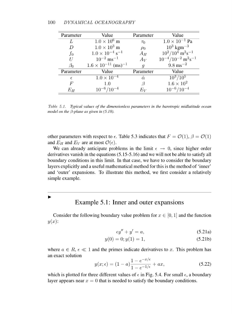
Table 5.1. Typical values of the dimensionless parameters in the barotropic midlatitude ocean
model on the β-plane as given in (5.18).
other parameters with respect to ǫ. Table 5.3 indicates that F = O(1), β = O(1)
and E H and E V are at most O(ǫ).
We can already anticipate problems in the limit ǫ → 0, since higher order
derivatives vanish in the equations (5.15-5.16) and we will not be able to satisfy all
boundary conditions in this limit. In that case, we have to consider the boundary
layers explicitly and a useful mathematical method for this is the method of ‘inner’
and ‘outer’ expansions. To illustrate this method, we first consider a relatively
simple example.
◮
Example 5.1: Inner and outer expansions
Consider the following boundary value problem for x ∈ [0, 1] and the function
y(x):
ǫy
′′ + y
′ = a,
(5.21a)
y(0) = 0; y(1) = 1,
(5.21b)
where a ∈ R, ǫ ≪ 1 and the primes indicate derivatives to x. This problem has
an exact solution
y(x; ǫ)=(1− a)
1 − e −x/ǫ
1 − e −1/ǫ + ax,
(5.22)
which is plotted for three different values of ǫ in Fig. 5.4. For small ǫ, a boundary
layer appears near x =0that is needed to satisfy the boundary conditions.
DYNAMICAL OCEANOGRAPHY
Parameter
Value
Parameter
Value
L
1.0 × 10 6 m
τ 0
1.0 × 10 −1 Pa
D
1.0 × 10 3 m
ρ 0
10 3 kgm −3
f 0
1.0 × 10 −4 s −1
A H
10 2 /10 4 m 2 s −1
U
10 −2 ms −1
A V
10 −4 /10 −2 m 2 s −1
β 0
1.6 × 10 −11 (ms) −1
g
9.8 ms −2
Parameter
Value
Parameter
Value
ǫ
1.0 × 10 −4
ˆ
α
10 3 /10 5
F
1.0
β
1.6 × 10 2
E H
10 −6 /10 −4
E V
10 −6 /10 −4
Table 5.1. Typical values of the dimensionless parameters in the barotropic midlatitude ocean
model on the β-plane as given in (5.18).
other parameters with respect to ǫ. Table 5.3 indicates that F = O(1), β = O(1)
and E H and E V are at most O(ǫ).
We can already anticipate problems in the limit ǫ → 0, since higher order
derivatives vanish in the equations (5.15-5.16) and we will not be able to satisfy all
boundary conditions in this limit. In that case, we have to consider the boundary
layers explicitly and a useful mathematical method for this is the method of ‘inner’
and ‘outer’ expansions. To illustrate this method, we first consider a relatively
simple example.
◮
Example 5.1: Inner and outer expansions
Consider the following boundary value problem for x ∈ [0, 1] and the function
y(x):
ǫy
′′ + y
′ = a,
(5.21a)
y(0) = 0; y(1) = 1,
(5.21b)
where a ∈ R, ǫ ≪ 1 and the primes indicate derivatives to x. This problem has
an exact solution
y(x; ǫ)=(1− a)
1 − e −x/ǫ
1 − e −1/ǫ + ax,
(5.22)
which is plotted for three different values of ǫ in Fig. 5.4. For small ǫ, a boundary
layer appears near x =0that is needed to satisfy the boundary conditions.