

Wind-driven circulation
99
F =
f 2
0 L 2
gD
; E H =
A H
f 0 L 2 ; E V =
A V
f 0 D 2 .
(5.18)
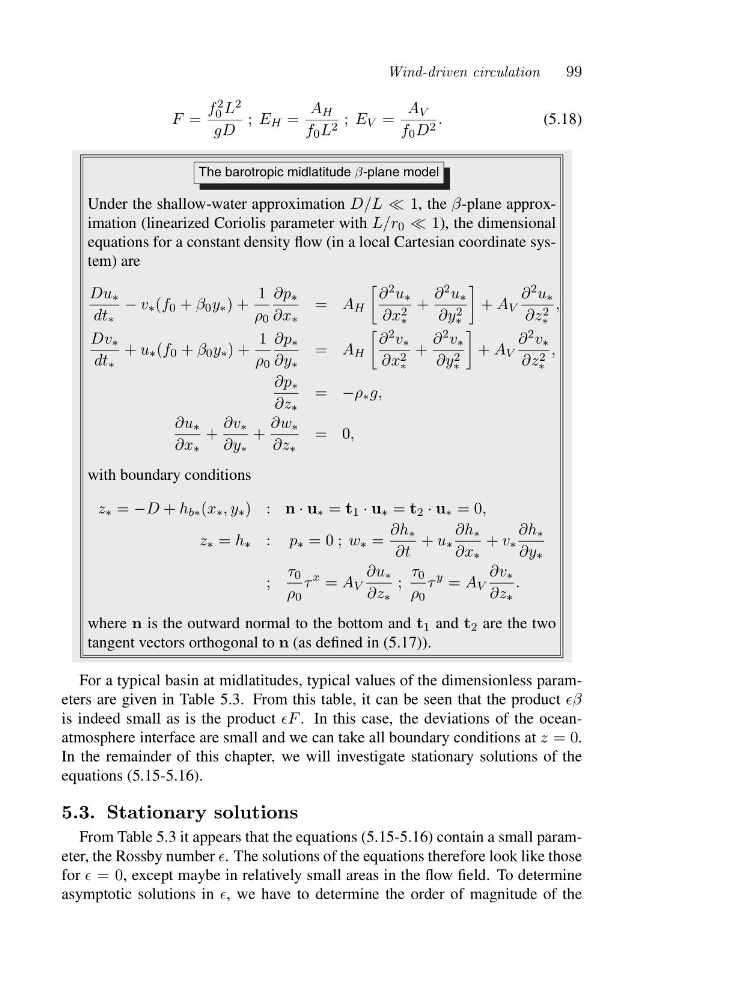
The barotropic midlatitude β-plane model
Under the shallow-water approximation D/L ≪ 1,t h eβ-plane approximation (linearized Coriolis parameter with L/r 0 ≪ 1), the dimensional
equations for a constant density flow (in a local Cartesian coordinate system) are
Du ∗
dt ∗
− v ∗ (f 0 + β 0 y ∗ )+
1
ρ 0
∂p ∗
∂x ∗
= A H
∂ 2 u ∗
∂x 2
∗
+
∂ 2 u ∗
∂y 2
∗
+ A V
∂ 2 u ∗
∂z 2
∗
,
Dv ∗
dt ∗
+ u ∗ (f 0 + β 0 y ∗ )+
1
ρ 0
∂p ∗
∂y ∗
= A H
∂ 2 v ∗
∂x 2
∗
+
∂ 2 v ∗
∂y 2
∗
+ A V
∂ 2 v ∗
∂z 2
∗
,
∂p ∗
∂z ∗
= −ρ ∗ g,
∂u ∗
∂x ∗
+
∂v ∗
∂y ∗
+
∂w ∗
∂z ∗
=0 ,
with boundary conditions
z ∗ = −D + h b∗ (x ∗ ,y ∗ ):n · u ∗ = t 1 · u ∗ = t 2 · u ∗ =0,
z ∗ = h ∗ : p ∗ =0; w ∗ =
∂h ∗
∂t
+ u ∗
∂h ∗
∂x ∗
+ v ∗
∂h ∗
∂y ∗
;
τ 0
ρ 0
τ
x = A V
∂u ∗
∂z ∗
;
τ 0
ρ 0
τ
y = A V
∂v ∗
∂z ∗
.
where n is the outward normal to the bottom and t 1 and t 2 are the two
tangent vectors orthogonal to n (as defined in (5.17)).
For a typical basin at midlatitudes, typical values of the dimensionless parameters are given in Table 5.3. From this table, it can be seen that the product ǫβ
is indeed small as is the product ǫF . In this case, the deviations of the oceanatmosphere interface are small and we can take all boundary conditions at z =0.
In the remainder of this chapter, we will investigate stationary solutions of the
equations (5.15-5.16).
5.3. Stationary solutions
From Table 5.3 it appears that the equations (5.15-5.16) contain a small parameter, the Rossby number ǫ. The solutions of the equations therefore look like those
for ǫ =0 , except maybe in relatively small areas in the flow field. To determine
asymptotic solutions in ǫ, we have to determine the order of magnitude of the
99
F =
f 2
0 L 2
gD
; E H =
A H
f 0 L 2 ; E V =
A V
f 0 D 2 .
(5.18)
The barotropic midlatitude β-plane model
Under the shallow-water approximation D/L ≪ 1,t h eβ-plane approximation (linearized Coriolis parameter with L/r 0 ≪ 1), the dimensional
equations for a constant density flow (in a local Cartesian coordinate system) are
Du ∗
dt ∗
− v ∗ (f 0 + β 0 y ∗ )+
1
ρ 0
∂p ∗
∂x ∗
= A H
∂ 2 u ∗
∂x 2
∗
+
∂ 2 u ∗
∂y 2
∗
+ A V
∂ 2 u ∗
∂z 2
∗
,
Dv ∗
dt ∗
+ u ∗ (f 0 + β 0 y ∗ )+
1
ρ 0
∂p ∗
∂y ∗
= A H
∂ 2 v ∗
∂x 2
∗
+
∂ 2 v ∗
∂y 2
∗
+ A V
∂ 2 v ∗
∂z 2
∗
,
∂p ∗
∂z ∗
= −ρ ∗ g,
∂u ∗
∂x ∗
+
∂v ∗
∂y ∗
+
∂w ∗
∂z ∗
=0 ,
with boundary conditions
z ∗ = −D + h b∗ (x ∗ ,y ∗ ):n · u ∗ = t 1 · u ∗ = t 2 · u ∗ =0,
z ∗ = h ∗ : p ∗ =0; w ∗ =
∂h ∗
∂t
+ u ∗
∂h ∗
∂x ∗
+ v ∗
∂h ∗
∂y ∗
;
τ 0
ρ 0
τ
x = A V
∂u ∗
∂z ∗
;
τ 0
ρ 0
τ
y = A V
∂v ∗
∂z ∗
.
where n is the outward normal to the bottom and t 1 and t 2 are the two
tangent vectors orthogonal to n (as defined in (5.17)).
For a typical basin at midlatitudes, typical values of the dimensionless parameters are given in Table 5.3. From this table, it can be seen that the product ǫβ
is indeed small as is the product ǫF . In this case, the deviations of the oceanatmosphere interface are small and we can take all boundary conditions at z =0.
In the remainder of this chapter, we will investigate stationary solutions of the
equations (5.15-5.16).
5.3. Stationary solutions
From Table 5.3 it appears that the equations (5.15-5.16) contain a small parameter, the Rossby number ǫ. The solutions of the equations therefore look like those
for ǫ =0 , except maybe in relatively small areas in the flow field. To determine
asymptotic solutions in ǫ, we have to determine the order of magnitude of the