

Wind-driven circulation
101
0
0.2
0.4
0.6
0.8
1
0
0.2
0.4
0.6
0.8
1
y
x
0.1
0.01
0.001
(a)
0
0.2
0.4
0.6
0.8
1
0
0.02
0.04
0.06
0.08
0.1
y
x
0.1
0.01
0.001
(b)
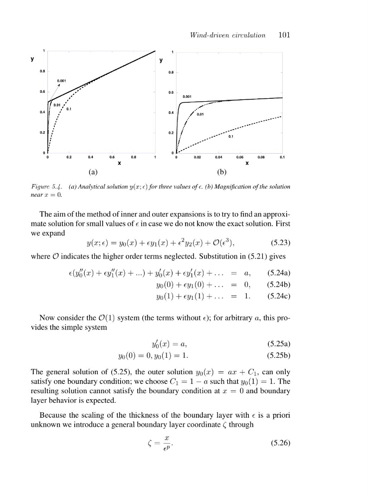
Figure 5.4. (a) Analytical solution y(x; ǫ) for three values of ǫ. (b) Magnification of the solution
near x =0.
The aim of the method of inner and outer expansions is to try to find an approximate solution for small values of ǫ in case we do not know the exact solution. First
we expand
y(x; ǫ)=y 0 (x)+ǫy 1 (x)+ǫ
2 y 2 (x)+O(ǫ
3 ),
(5.23)
where O indicates the higher order terms neglected. Substitution in (5.21) gives
ǫ(y
′′
0 (x)+ǫy
′′
1 (x)+...)+y
′
0 (x)+ǫy
′
1 (x)+... = a,
(5.24a)
y 0 (0) + ǫy 1 (0) + ... =0 ,
(5.24b)
y 0 (1) + ǫy 1 (1) + ... =1 .
(5.24c)
Now consider the O(1) system (the terms without ǫ); for arbitrary a,thisprovides the simple system
y
′
0 (x)=a,
(5.25a)
y 0 (0) = 0,y 0 (1) = 1.
(5.25b)
The general solution of (5.25), the outer solution y 0 (x)=ax + C 1 , can only
satisfy one boundary condition; we choose C 1 =1− a such that y 0 (1) = 1.T h e
resulting solution cannot satisfy the boundary condition at x =0and boundary
layer behavior is expected.
Because the scaling of the thickness of the boundary layer with ǫ is a priori
unknown we introduce a general boundary layer coordinate ζ through
ζ =
x
ǫ p .
(5.26)
101
0
0.2
0.4
0.6
0.8
1
0
0.2
0.4
0.6
0.8
1
y
x
0.1
0.01
0.001
(a)
0
0.2
0.4
0.6
0.8
1
0
0.02
0.04
0.06
0.08
0.1
y
x
0.1
0.01
0.001
(b)
Figure 5.4. (a) Analytical solution y(x; ǫ) for three values of ǫ. (b) Magnification of the solution
near x =0.
The aim of the method of inner and outer expansions is to try to find an approximate solution for small values of ǫ in case we do not know the exact solution. First
we expand
y(x; ǫ)=y 0 (x)+ǫy 1 (x)+ǫ
2 y 2 (x)+O(ǫ
3 ),
(5.23)
where O indicates the higher order terms neglected. Substitution in (5.21) gives
ǫ(y
′′
0 (x)+ǫy
′′
1 (x)+...)+y
′
0 (x)+ǫy
′
1 (x)+... = a,
(5.24a)
y 0 (0) + ǫy 1 (0) + ... =0 ,
(5.24b)
y 0 (1) + ǫy 1 (1) + ... =1 .
(5.24c)
Now consider the O(1) system (the terms without ǫ); for arbitrary a,thisprovides the simple system
y
′
0 (x)=a,
(5.25a)
y 0 (0) = 0,y 0 (1) = 1.
(5.25b)
The general solution of (5.25), the outer solution y 0 (x)=ax + C 1 , can only
satisfy one boundary condition; we choose C 1 =1− a such that y 0 (1) = 1.T h e
resulting solution cannot satisfy the boundary condition at x =0and boundary
layer behavior is expected.
Because the scaling of the thickness of the boundary layer with ǫ is a priori
unknown we introduce a general boundary layer coordinate ζ through
ζ =
x
ǫ p .
(5.26)