

62
N. Makarenko et al.
í µí»¼ 1 (í µí¼) =
í µí¼ + í µí¼
√
í µí¼F 1
, í µí»¼ 2 (í µí¼) =
í µí¼ − rí µí¼
√
í µí¼F 2
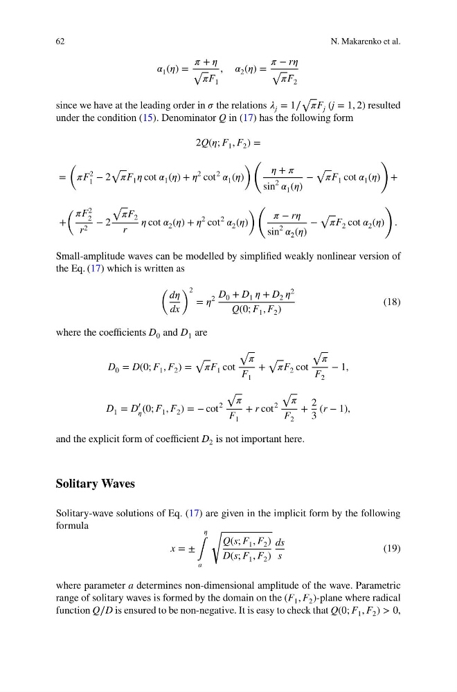
since we have at the leading order in í µí¼ the relations í µí¼ j = 1∕
√
í µí¼F j (j = 1, 2) resulted
under the condition (15). Denominator Q in (17) has the following form
2Q(í µí¼; F 1 , F 2 ) =
=
(
í µí¼F
2
1 − 2
√ í µí¼F 1 í µí¼ cot í µí»¼ 1 (í µí¼) + í µí¼
2
cot
2
í µí»¼ 1 (í µí¼)
) (
í µí¼ + í µí¼
sin
2
í µí»¼ 1 (í µí¼)
−
√
í µí¼F 1 cot í µí»¼ 1 (í µí¼)
)
+
+
( í µí¼F
2
2
r 2 − 2
√
í µí¼F 2
r
í µí¼ cot í µí»¼ 2 (í µí¼) + í µí¼
2
cot
2
í µí»¼ 2 (í µí¼)
) (
í µí¼ − rí µí¼
sin
2
í µí»¼ 2 (í µí¼)
−
√
í µí¼F 2 cot í µí»¼ 2 (í µí¼)
)
.
Small-amplitude waves can be modelled by simplified weakly nonlinear version of
the Eq. (17) which is written as
(
dí µí¼
dx
) 2
= í µí¼
2 D 0 + D 1 í µí¼ + D 2 í µí¼ 2
Q(0; F 1 , F 2 )
(18)
where the coefficients D 0 and D 1 are
D 0 = D(0; F 1 , F 2 ) =
√
í µí¼F 1 cot
√
í µí¼
F 1
+
√
í µí¼F 2 cot
√ í µí¼
F 2
− 1,
D 1 = D
′
í µí¼ (0; F 1 , F 2 ) = − cot
2
√ í µí¼
F 1
+ r cot
2
√
í µí¼
F 2
+
2
3
(r − 1),
and the explicit form of coefficient D 2 is not important here.
Solitary Waves
Solitary-wave solutions of Eq. (17) are given in the implicit form by the following
formula
x = ±
í µí¼
∫
a
√
Q(s; F 1 , F 2 )
D(s; F 1 , F 2 )
ds
s
(19)
where parameter a determines non-dimensional amplitude of the wave. Parametric
range of solitary waves is formed by the domain on the (F 1 , F 2 )-plane where radical
function Q∕D is ensured to be non-negative. It is easy to check that Q(0; F 1 , F 2 ) > 0,
N. Makarenko et al.
í µí»¼ 1 (í µí¼) =
í µí¼ + í µí¼
√
í µí¼F 1
, í µí»¼ 2 (í µí¼) =
í µí¼ − rí µí¼
√
í µí¼F 2
since we have at the leading order in í µí¼ the relations í µí¼ j = 1∕
√
í µí¼F j (j = 1, 2) resulted
under the condition (15). Denominator Q in (17) has the following form
2Q(í µí¼; F 1 , F 2 ) =
=
(
í µí¼F
2
1 − 2
√ í µí¼F 1 í µí¼ cot í µí»¼ 1 (í µí¼) + í µí¼
2
cot
2
í µí»¼ 1 (í µí¼)
) (
í µí¼ + í µí¼
sin
2
í µí»¼ 1 (í µí¼)
−
√
í µí¼F 1 cot í µí»¼ 1 (í µí¼)
)
+
+
( í µí¼F
2
2
r 2 − 2
√
í µí¼F 2
r
í µí¼ cot í µí»¼ 2 (í µí¼) + í µí¼
2
cot
2
í µí»¼ 2 (í µí¼)
) (
í µí¼ − rí µí¼
sin
2
í µí»¼ 2 (í µí¼)
−
√
í µí¼F 2 cot í µí»¼ 2 (í µí¼)
)
.
Small-amplitude waves can be modelled by simplified weakly nonlinear version of
the Eq. (17) which is written as
(
dí µí¼
dx
) 2
= í µí¼
2 D 0 + D 1 í µí¼ + D 2 í µí¼ 2
Q(0; F 1 , F 2 )
(18)
where the coefficients D 0 and D 1 are
D 0 = D(0; F 1 , F 2 ) =
√
í µí¼F 1 cot
√
í µí¼
F 1
+
√
í µí¼F 2 cot
√ í µí¼
F 2
− 1,
D 1 = D
′
í µí¼ (0; F 1 , F 2 ) = − cot
2
√ í µí¼
F 1
+ r cot
2
√
í µí¼
F 2
+
2
3
(r − 1),
and the explicit form of coefficient D 2 is not important here.
Solitary Waves
Solitary-wave solutions of Eq. (17) are given in the implicit form by the following
formula
x = ±
í µí¼
∫
a
√
Q(s; F 1 , F 2 )
D(s; F 1 , F 2 )
ds
s
(19)
where parameter a determines non-dimensional amplitude of the wave. Parametric
range of solitary waves is formed by the domain on the (F 1 , F 2 )-plane where radical
function Q∕D is ensured to be non-negative. It is easy to check that Q(0; F 1 , F 2 ) > 0,