

was the presence of a linear gradient on the vertical profiles within the water layer
10 m above and below the level that was under the consideration. Part of measurements at the levels was not transformed to vertical displacements and was not
used in the calculation of frequency spectra. It happened in the cases when there
were such reorganizations of the structure of vertical gradients on consecutive
vertical profiles, which eventually formed a nonlinear gradient in the neighborhood
of these levels. It should be noted that only about 2% of the records at the levels
were subjected to such rejection since the measurements were made within the
northern part of the Amundsen Basin where the horizontal TS fields are comparatively uniform because of their location far from the frontal zones or others causes
of abrupt changes in the halocline or thermocline.
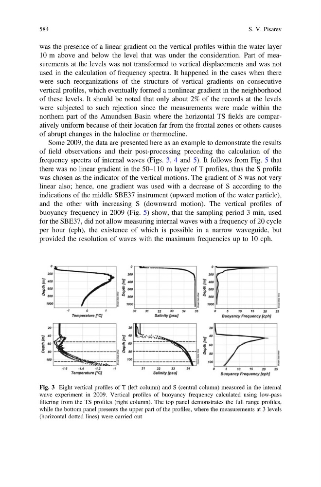
Some 2009, the data are presented here as an example to demonstrate the results
of field observations and their post-processing preceding the calculation of the
frequency spectra of internal waves (Figs. 3, 4 and 5). It follows from Fig. 5 that
there was no linear gradient in the 50–110 m layer of T profiles, thus the S profile
was chosen as the indicator of the vertical motions. The gradient of S was not very
linear also; hence, one gradient was used with a decrease of S according to the
indications of the middle SBE37 instrument (upward motion of the water particle),
and the other with increasing S (downward motion). The vertical profiles of
buoyancy frequency in 2009 (Fig. 5) show, that the sampling period 3 min, used
for the SBE37, did not allow measuring internal waves with a frequency of 20 cycle
per hour (cph), the existence of which is possible in a narrow waveguide, but
provided the resolution of waves with the maximum frequencies up to 10 cph.
Fig. 3 Eight vertical profiles of T (left column) and S (central column) measured in the internal
wave experiment in 2009. Vertical profiles of buoyancy frequency calculated using low-pass
filtering from the TS profiles (right column). The top panel demonstrates the full range profiles,
while the bottom panel presents the upper part of the profiles, where the measurements at 3 levels
(horizontal dotted lines) were carried out
584
S. V. Pisarev