

46
J. Grue
Figure 1 plots the resistance coefficient (4) as function of the speed U 2 in the dead
water, for the two different ship speeds U 1 without dead water, of 5 knots or 4.5 knots,
corresponding to the range given in Ekman [2]. The dead water resistance coefficient
is divided by the ratio between the ship draught and upper layer depth squared, i.e.
(b 0 ∕h 0 )
2 . While the draught of the FRAM was b 0 = 5 m, the mid depth of the
pycnocline was most possibly located at h 0 = 4 m depth (or somewhat shallower).
In the calculations below we find it convenient to calculate the dead water resistance
coefficient divided by (b 0 ∕h 0 )
2 where the nonlinear interfacial calculations in section
“Nonlinear Interfacial Model” and section “Dead Water Resistance” are obtained
for the range 0.8 ≤ b 0 ∕h 1 ≤ 1 of the nondimensional draught and where values for
the actual draught of b 0 ∕h 0 = 5∕4 are obtained by extrapolation. The level of the
pycnocline is further elaborated on in section “Upper Layer Depth. Draught of Ship
Model” below.
Nonlinear Interfacial Model
The interaction between the ship moving at forward speed U and the stratified sea is
here modelled assuming a two-layer fluid, with the pycnocline replaced by an interface. This is a good approximation when the internal wavelength is great compared
to the pycnocline thickness [15]. The two-layer model favourably compares with a
three-layer model regarding the wave speeds and wave patterns in the dead water
problem [12]. The Froude number of the surface waves based on the ship length, of
U∕
√
gl 0 ≪ 1, justifies the rigid lid condition at the upper boundary of the fluid layer.
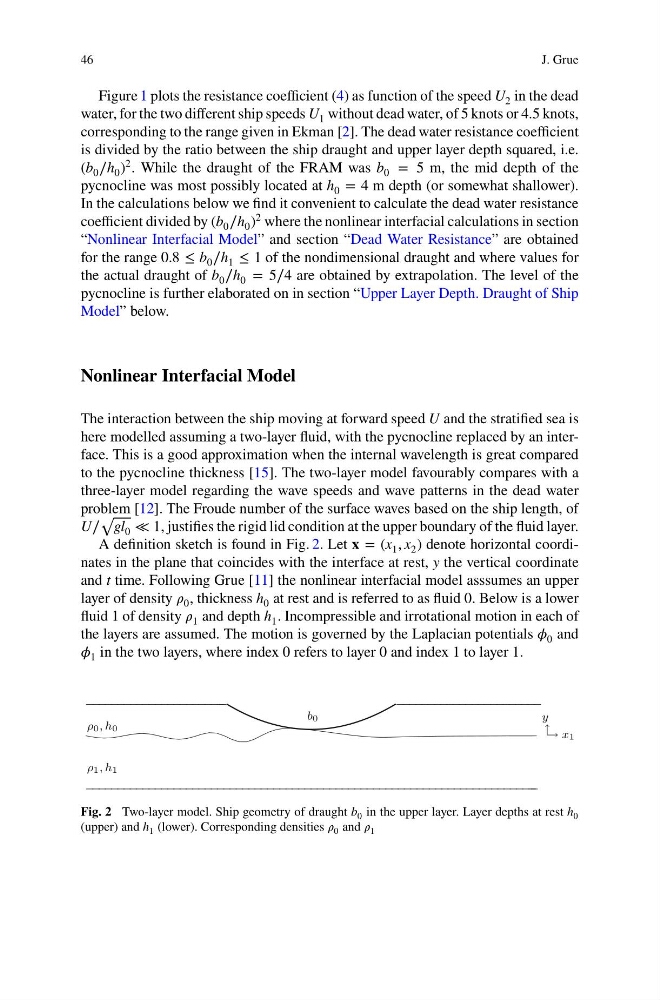
A definition sketch is found in Fig. 2. Let í µí°± = (x 1 , x 2 ) denote horizontal coordinates in the plane that coincides with the interface at rest, y the vertical coordinate
and t time. Following Grue [11] the nonlinear interfacial model asssumes an upper
layer of density í µí¼ 0 , thickness h 0 at rest and is referred to as fluid 0. Below is a lower
fluid 1 of density í µí¼ 1 and depth h 1 . Incompressible and irrotational motion in each of
the layers are assumed. The motion is governed by the Laplacian potentials í µí¼ 0 and
í µí¼ 1 in the two layers, where index 0 refers to layer 0 and index 1 to layer 1.
ρ 0 , h 0
ρ 1 , h 1
→ x 1
↑
y
b 0
−−−−−−−−−−−−−−−−−−−−−− −
− −−−−−−−−−−−−−−−−−−−−−−
Fig. 2 Two-layer model. Ship geometry of draught b 0 in the upper layer. Layer depths at rest h 0
(upper) and h 1 (lower). Corresponding densities í µí¼ 0 and í µí¼ 1
J. Grue
Figure 1 plots the resistance coefficient (4) as function of the speed U 2 in the dead
water, for the two different ship speeds U 1 without dead water, of 5 knots or 4.5 knots,
corresponding to the range given in Ekman [2]. The dead water resistance coefficient
is divided by the ratio between the ship draught and upper layer depth squared, i.e.
(b 0 ∕h 0 )
2 . While the draught of the FRAM was b 0 = 5 m, the mid depth of the
pycnocline was most possibly located at h 0 = 4 m depth (or somewhat shallower).
In the calculations below we find it convenient to calculate the dead water resistance
coefficient divided by (b 0 ∕h 0 )
2 where the nonlinear interfacial calculations in section
“Nonlinear Interfacial Model” and section “Dead Water Resistance” are obtained
for the range 0.8 ≤ b 0 ∕h 1 ≤ 1 of the nondimensional draught and where values for
the actual draught of b 0 ∕h 0 = 5∕4 are obtained by extrapolation. The level of the
pycnocline is further elaborated on in section “Upper Layer Depth. Draught of Ship
Model” below.
Nonlinear Interfacial Model
The interaction between the ship moving at forward speed U and the stratified sea is
here modelled assuming a two-layer fluid, with the pycnocline replaced by an interface. This is a good approximation when the internal wavelength is great compared
to the pycnocline thickness [15]. The two-layer model favourably compares with a
three-layer model regarding the wave speeds and wave patterns in the dead water
problem [12]. The Froude number of the surface waves based on the ship length, of
U∕
√
gl 0 ≪ 1, justifies the rigid lid condition at the upper boundary of the fluid layer.
A definition sketch is found in Fig. 2. Let í µí°± = (x 1 , x 2 ) denote horizontal coordinates in the plane that coincides with the interface at rest, y the vertical coordinate
and t time. Following Grue [11] the nonlinear interfacial model asssumes an upper
layer of density í µí¼ 0 , thickness h 0 at rest and is referred to as fluid 0. Below is a lower
fluid 1 of density í µí¼ 1 and depth h 1 . Incompressible and irrotational motion in each of
the layers are assumed. The motion is governed by the Laplacian potentials í µí¼ 0 and
í µí¼ 1 in the two layers, where index 0 refers to layer 0 and index 1 to layer 1.
ρ 0 , h 0
ρ 1 , h 1
→ x 1
↑
y
b 0
−−−−−−−−−−−−−−−−−−−−−− −
− −−−−−−−−−−−−−−−−−−−−−−
Fig. 2 Two-layer model. Ship geometry of draught b 0 in the upper layer. Layer depths at rest h 0
(upper) and h 1 (lower). Corresponding densities í µí¼ 0 and í µí¼ 1