Calculating FRAM’s Dead Water
47
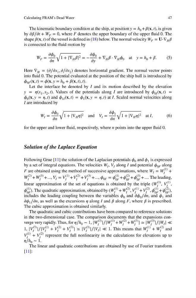
The kinematic boundary condition at the ship, at position y = h 0 +𝛽(𝐱, t), is given
by 𝜕𝛽∕𝜕t + W F = 0, where F denotes the upper boundary of the upper fluid 0. The
shape 𝛽(𝐱, t) of the vessel is defined in (18) below. The normal velocity W F = 𝐔⋅∇ H 𝛽
is connected to the fluid motion by
W F =
𝜕𝜙 0
𝜕n
√
1 + |∇ H 𝛽| 2 = −
𝜕𝜙 0
𝜕y
+ ∇ H 𝛽 ⋅ ∇ H 𝜙 0 at y = h 0 + 𝛽.
(5)
Here ∇ H = (𝜕∕𝜕x 1 , 𝜕∕𝜕x 2 ) denotes horizontal gradient. The normal vector points
into fluid 0. The potential evaluated at the position of the ship hull is introduced by
𝜙 0F (𝐱, t) = 𝜙(𝐱, y = h 0 + 𝛽(𝐱, t), t).
Let the interface be denoted by I and its motion described by the elevation
y = 𝜂(x 1 , x 2 , t). Values of the potentials along I are introduced by 𝜙 0I (𝐱, t) =
𝜙 0 (𝐱, y = 𝜂, t) and 𝜙 1I (𝐱, t) = 𝜙 1 (𝐱, y = 𝜂, t) at I. Scaled normal velocities along
I are introduced by
W I =
𝜕𝜙 0
𝜕n
√
1 + |∇ H 𝜂| 2 and V I =
𝜕𝜙 1
𝜕n
√
1 + |∇ H 𝜂| 2 at I,
( 6 )
for the upper and lower fluid, respectively, where n points into the upper fluid 0.
Solution of the Laplace Equation
Following Grue [11] the solution of the Laplacian potentials 𝜙 0 and 𝜙 1 is expressed
by a set of integral equations. The velocities W I , V I along I and potential 𝜙 0F along
F are obtained using the method of successive approximations, where W I = W
(1)
I
+
W
(2)
I
+W
(3)
I
+..., V I = V
(1)
I
+V
(2)
I
+V
(3)
I
+..., 𝜙 0F = 𝜙
(1)
0F
+𝜙
(2)
0F
+𝜙
(3)
0F
+.... The leading,
linear approximation of the set of equations is obtained by the triple (W
(1)
I
, V
(1)
I
,
𝜙
(1)
0F
). The quadratic approximation, obtained by (W
(1)
I
+ W
(2)
I
, V
(1)
I
+ V
(2)
I
, 𝜙
(1)
0F
+ 𝜙
(2)
0F
),
includes the leading coupling between the variables 𝜙 0 and 𝜕𝜙 0 ∕𝜕n, and 𝜙 1 and
𝜕𝜙 1 ∕𝜕n, as well as the excursions 𝜂 along I and 𝛽 along F, where 𝛽 is prescribed.
The cubic approximation is obtained similarly.
The quadratic and cubic contributions have been compared to reference solutions
in the two-dimensional case. The comparison documents that the expansions converge very rapidly. Thus, for 𝜂∕h 0 ∼ 1, |W
(3)
I
|∕|W
(1)
I
+W
(2)
I
+W
(3)
I
| ≃ |W
(3)
I
|∕|W I | ≪
1, |V
(3)
I
|∕|V
(1)
I
+ V
(2)
I
+ V
(3)
I
| ≃ |V
(3)
I
|∕|V I | ≪ 1. This means that W
(1)
I
+ W
(2)
I
and
V
(1)
I
+ V
(2)
I
represent the full nonlinearity in the calculations for elevations up to
𝜂∕h 0 ∼ 1.
The linear and quadratic contributions are obtained by use of Fourier transform
[11]: