

3 years (2012–2014) the model has been integrated with the correction each
3 months according to formulae (1) and (3), then again it has been integrated free
until 2016. The observations were included at the end of each 3-month period;
previously they have been smoothed with 11-point filter along the track. In parallel,
the reference experiment, i.e. integration without correction has been performed
over the entire period 2010–2016.
Analysis of the computed geophysical fields is presented below. The sea level is
the integral variable, which means that its variability stems from the integral
variability of many other variables both in the atmosphere and in the ocean, such as
wind stress, thermal expansion, precipitation, and many others. This leads to the
fact that the assimilation of the sea level implies the changing of many other
variables; hence, it will affect the entire system forming the sea level. These processes are very complex; however, one can see the model output of all characteristics after a specific period of model integration. Among the output parameters the
sea level fields were the direct output, but we also analyzed the ice thickness and ice
concentration. Special attention was focused on the Arctic zone of Russia.
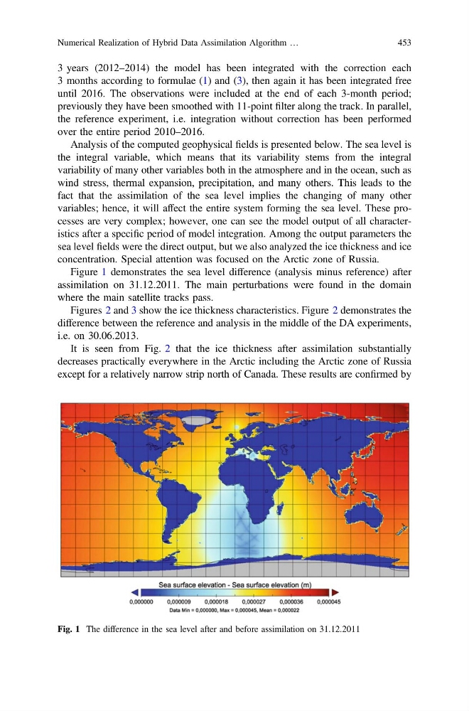
Figure 1 demonstrates the sea level difference (analysis minus reference) after
assimilation on 31.12.2011. The main perturbations were found in the domain
where the main satellite tracks pass.
Figures 2 and 3 show the ice thickness characteristics. Figure 2 demonstrates the
difference between the reference and analysis in the middle of the DA experiments,
i.e. on 30.06.2013.
It is seen from Fig. 2 that the ice thickness after assimilation substantially
decreases practically everywhere in the Arctic including the Arctic zone of Russia
except for a relatively narrow strip north of Canada. These results are confirmed by
Fig. 1 The difference in the sea level after and before assimilation on 31.12.2011
Numerical Realization of Hybrid Data Assimilation Algorithm …
453
3 months according to formulae (1) and (3), then again it has been integrated free
until 2016. The observations were included at the end of each 3-month period;
previously they have been smoothed with 11-point filter along the track. In parallel,
the reference experiment, i.e. integration without correction has been performed
over the entire period 2010–2016.
Analysis of the computed geophysical fields is presented below. The sea level is
the integral variable, which means that its variability stems from the integral
variability of many other variables both in the atmosphere and in the ocean, such as
wind stress, thermal expansion, precipitation, and many others. This leads to the
fact that the assimilation of the sea level implies the changing of many other
variables; hence, it will affect the entire system forming the sea level. These processes are very complex; however, one can see the model output of all characteristics after a specific period of model integration. Among the output parameters the
sea level fields were the direct output, but we also analyzed the ice thickness and ice
concentration. Special attention was focused on the Arctic zone of Russia.
Figure 1 demonstrates the sea level difference (analysis minus reference) after
assimilation on 31.12.2011. The main perturbations were found in the domain
where the main satellite tracks pass.
Figures 2 and 3 show the ice thickness characteristics. Figure 2 demonstrates the
difference between the reference and analysis in the middle of the DA experiments,
i.e. on 30.06.2013.
It is seen from Fig. 2 that the ice thickness after assimilation substantially
decreases practically everywhere in the Arctic including the Arctic zone of Russia
except for a relatively narrow strip north of Canada. These results are confirmed by
Fig. 1 The difference in the sea level after and before assimilation on 31.12.2011
Numerical Realization of Hybrid Data Assimilation Algorithm …
453