

scheme to calculate this matrix is the Monte-Carlo method, which is widely used in
the Kalman-filter theory [5]. The issue to calculate this matrix optimally is also
beyond the consideration of the current work.
Numerical Experiments and their Results
The numerical experiments with the MPIESM model in conjunction with the DA
scheme (1)–(3) have been performed.
The ocean block is the MPIOM model (version 1.2) with a resolution of
256 × 220 × 40 grid points, by longitude, latitude, and vertical direction,
respectively. The resolution is not uniform, it is fine in the high latitude domain and
in the upper ocean levels; it is coarse in the Southern Ocean and in the deep layers.
In the Arctic zone, the horizontal grid mesh is about 30 km. In the ocean model
block, ice dynamics and confluence module are developed specially. A full
description is presented in the model manual, which can be found in [8, 13]. The
atmosphere block represents the ECHAM6 model. Its resolution is T63L47 (the
spectrum model with 63 basis eigenfunctions and 47 vertical levels), which regards
to approximately 240 km of the spatial grid distance. The ocean-atmosphere
interaction is realized through the OASIS block.
Initialization of the model has been forced from climate Atlas NCEP (URL:
http://www.cpc.ncep.noaa.gov/products/precip/atlas_2/cont_data.html), and the
spin up run has been performed to establish the constant energy regime of the
currents in the ocean from 1850 to 2010. The date 01.01.2010 was set up as the
initial date for the further DA experiments.
Several numerical experiments have been carried out with the DA, in which the
model result has been corrected by formulae (1) and (3), while the observed data of
the sea level were taken from AVISO data. Vector C for the sea level has been set
up as interpolation onto the model grid points of the observed sea level minus
model sea level at the previous time-step. For other model variables the values were
taken as time average of the corresponding variables minus their model value on the
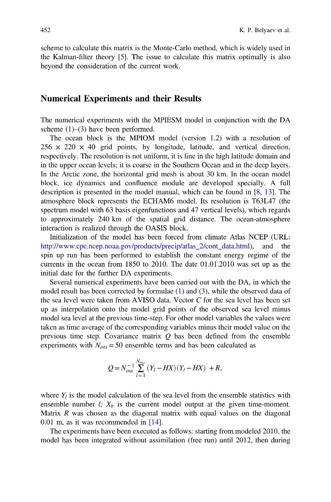
previous time step. Covariance matrix Q has been defined from the ensemble
experiments with N ens = 50 ensemble terms and has been calculated as
Q = N
− 1
ens ∑
N ens
l = 1
ðY l − HXÞðY l − HXÞ
′ + R,
where Y l is the model calculation of the sea level from the ensemble statistics with
ensemble number l; X b is the current model output at the given time-moment.
Matrix R was chosen as the diagonal matrix with equal values on the diagonal
0.01 m, as it was recommended in [14].
The experiments have been executed as follows: starting from modeled 2010, the
model has been integrated without assimilation (free run) until 2012, then during
452
K. P. Belyaev et al.
the Kalman-filter theory [5]. The issue to calculate this matrix optimally is also
beyond the consideration of the current work.
Numerical Experiments and their Results
The numerical experiments with the MPIESM model in conjunction with the DA
scheme (1)–(3) have been performed.
The ocean block is the MPIOM model (version 1.2) with a resolution of
256 × 220 × 40 grid points, by longitude, latitude, and vertical direction,
respectively. The resolution is not uniform, it is fine in the high latitude domain and
in the upper ocean levels; it is coarse in the Southern Ocean and in the deep layers.
In the Arctic zone, the horizontal grid mesh is about 30 km. In the ocean model
block, ice dynamics and confluence module are developed specially. A full
description is presented in the model manual, which can be found in [8, 13]. The
atmosphere block represents the ECHAM6 model. Its resolution is T63L47 (the
spectrum model with 63 basis eigenfunctions and 47 vertical levels), which regards
to approximately 240 km of the spatial grid distance. The ocean-atmosphere
interaction is realized through the OASIS block.
Initialization of the model has been forced from climate Atlas NCEP (URL:
http://www.cpc.ncep.noaa.gov/products/precip/atlas_2/cont_data.html), and the
spin up run has been performed to establish the constant energy regime of the
currents in the ocean from 1850 to 2010. The date 01.01.2010 was set up as the
initial date for the further DA experiments.
Several numerical experiments have been carried out with the DA, in which the
model result has been corrected by formulae (1) and (3), while the observed data of
the sea level were taken from AVISO data. Vector C for the sea level has been set
up as interpolation onto the model grid points of the observed sea level minus
model sea level at the previous time-step. For other model variables the values were
taken as time average of the corresponding variables minus their model value on the
previous time step. Covariance matrix Q has been defined from the ensemble
experiments with N ens = 50 ensemble terms and has been calculated as
Q = N
− 1
ens ∑
N ens
l = 1
ðY l − HXÞðY l − HXÞ
′ + R,
where Y l is the model calculation of the sea level from the ensemble statistics with
ensemble number l; X b is the current model output at the given time-moment.
Matrix R was chosen as the diagonal matrix with equal values on the diagonal
0.01 m, as it was recommended in [14].
The experiments have been executed as follows: starting from modeled 2010, the
model has been integrated without assimilation (free run) until 2012, then during
452
K. P. Belyaev et al.