

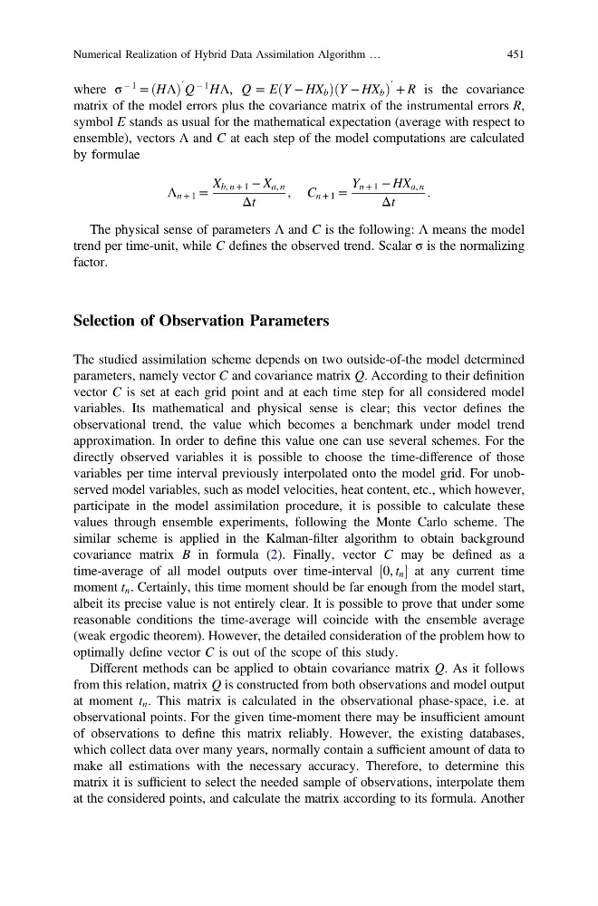
where σ
− 1 = ðHΛÞ
′ Q
− 1 HΛ, Q = EðY − HX b ÞðY − HX b Þ
′ + R is the covariance
matrix of the model errors plus the covariance matrix of the instrumental errors R,
symbol E stands as usual for the mathematical expectation (average with respect to
ensemble), vectors Λ and C at each step of the model computations are calculated
by formulae
Λ n + 1 =
X b, n + 1 − X a, n
Δt
, C n + 1 =
Y n + 1 − HX a, n
Δt
.
The physical sense of parameters Λ and C is the following: Λ means the model
trend per time-unit, while C defines the observed trend. Scalar σ is the normalizing
factor.
Selection of Observation Parameters
The studied assimilation scheme depends on two outside-of-the model determined
parameters, namely vector C and covariance matrix Q. According to their definition
vector C is set at each grid point and at each time step for all considered model
variables. Its mathematical and physical sense is clear; this vector defines the
observational trend, the value which becomes a benchmark under model trend
approximation. In order to define this value one can use several schemes. For the
directly observed variables it is possible to choose the time-difference of those
variables per time interval previously interpolated onto the model grid. For unobserved model variables, such as model velocities, heat content, etc., which however,
participate in the model assimilation procedure, it is possible to calculate these
values through ensemble experiments, following the Monte Carlo scheme. The
similar scheme is applied in the Kalman-filter algorithm to obtain background
covariance matrix B in formula (2). Finally, vector C may be defined as a
time-average of all model outputs over time-interval ½0, t n at any current time
moment t n . Certainly, this time moment should be far enough from the model start,
albeit its precise value is not entirely clear. It is possible to prove that under some
reasonable conditions the time-average will coincide with the ensemble average
(weak ergodic theorem). However, the detailed consideration of the problem how to
optimally define vector C is out of the scope of this study.
Different methods can be applied to obtain covariance matrix Q. As it follows
from this relation, matrix Q is constructed from both observations and model output
at moment t n . This matrix is calculated in the observational phase-space, i.e. at
observational points. For the given time-moment there may be insufficient amount
of observations to define this matrix reliably. However, the existing databases,
which collect data over many years, normally contain a sufficient amount of data to
make all estimations with the necessary accuracy. Therefore, to determine this
matrix it is sufficient to select the needed sample of observations, interpolate them
at the considered points, and calculate the matrix according to its formula. Another
Numerical Realization of Hybrid Data Assimilation Algorithm …
451
− 1 = ðHΛÞ
′ Q
− 1 HΛ, Q = EðY − HX b ÞðY − HX b Þ
′ + R is the covariance
matrix of the model errors plus the covariance matrix of the instrumental errors R,
symbol E stands as usual for the mathematical expectation (average with respect to
ensemble), vectors Λ and C at each step of the model computations are calculated
by formulae
Λ n + 1 =
X b, n + 1 − X a, n
Δt
, C n + 1 =
Y n + 1 − HX a, n
Δt
.
The physical sense of parameters Λ and C is the following: Λ means the model
trend per time-unit, while C defines the observed trend. Scalar σ is the normalizing
factor.
Selection of Observation Parameters
The studied assimilation scheme depends on two outside-of-the model determined
parameters, namely vector C and covariance matrix Q. According to their definition
vector C is set at each grid point and at each time step for all considered model
variables. Its mathematical and physical sense is clear; this vector defines the
observational trend, the value which becomes a benchmark under model trend
approximation. In order to define this value one can use several schemes. For the
directly observed variables it is possible to choose the time-difference of those
variables per time interval previously interpolated onto the model grid. For unobserved model variables, such as model velocities, heat content, etc., which however,
participate in the model assimilation procedure, it is possible to calculate these
values through ensemble experiments, following the Monte Carlo scheme. The
similar scheme is applied in the Kalman-filter algorithm to obtain background
covariance matrix B in formula (2). Finally, vector C may be defined as a
time-average of all model outputs over time-interval ½0, t n at any current time
moment t n . Certainly, this time moment should be far enough from the model start,
albeit its precise value is not entirely clear. It is possible to prove that under some
reasonable conditions the time-average will coincide with the ensemble average
(weak ergodic theorem). However, the detailed consideration of the problem how to
optimally define vector C is out of the scope of this study.
Different methods can be applied to obtain covariance matrix Q. As it follows
from this relation, matrix Q is constructed from both observations and model output
at moment t n . This matrix is calculated in the observational phase-space, i.e. at
observational points. For the given time-moment there may be insufficient amount
of observations to define this matrix reliably. However, the existing databases,
which collect data over many years, normally contain a sufficient amount of data to
make all estimations with the necessary accuracy. Therefore, to determine this
matrix it is sufficient to select the needed sample of observations, interpolate them
at the considered points, and calculate the matrix according to its formula. Another
Numerical Realization of Hybrid Data Assimilation Algorithm …
451