

In this study, the original hybrid scheme of the DA-method and several versions
of its application are presented and discussed. The coupled Max Plank Institute
Earth System model (MPIESM), developed at the Max Plank Institute for Meteorology in Hamburg [8, 13] is considered the main tool for the implementation of the
DA-scheme.
Data Assimilation Method
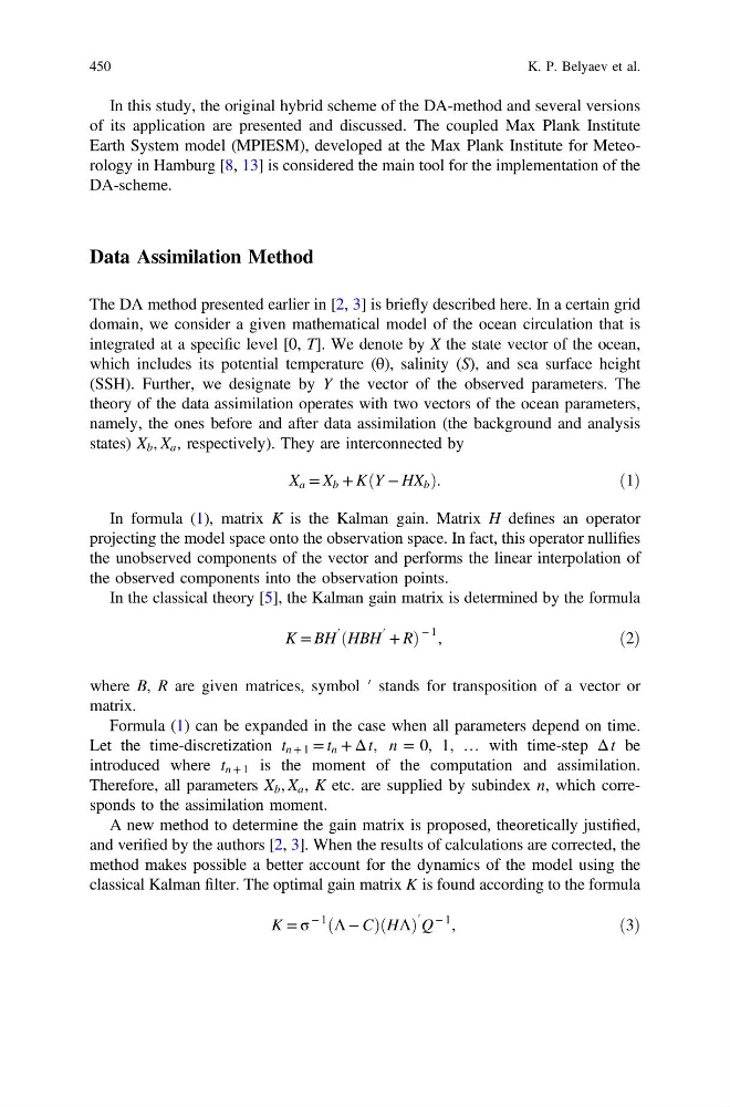
The DA method presented earlier in [2, 3] is briefly described here. In a certain grid
domain, we consider a given mathematical model of the ocean circulation that is
integrated at a specific level [0, T]. We denote by X the state vector of the ocean,
which includes its potential temperature (θ), salinity (S), and sea surface height
(SSH). Further, we designate by Y the vector of the observed parameters. The
theory of the data assimilation operates with two vectors of the ocean parameters,
namely, the ones before and after data assimilation (the background and analysis
states) X b , X a , respectively). They are interconnected by
X a = X b + KðY − HX b Þ.
ð1Þ
In formula (1), matrix K is the Kalman gain. Matrix H defines an operator
projecting the model space onto the observation space. In fact, this operator nullifies
the unobserved components of the vector and performs the linear interpolation of
the observed components into the observation points.
In the classical theory [5], the Kalman gain matrix is determined by the formula
K = BH
′
ðHBH
′ + RÞ
− 1 ,
ð2Þ
where B, R are given matrices, symbol ′ stands for transposition of a vector or
matrix.
Formula (1) can be expanded in the case when all parameters depend on time.
Let the time-discretization t n + 1 = t n + Δ t, n = 0, 1, … with time-step Δ t be
introduced where t n + 1 is the moment of the computation and assimilation.
Therefore, all parameters X b , X a , K etc. are supplied by subindex n, which corresponds to the assimilation moment.
A new method to determine the gain matrix is proposed, theoretically justified,
and verified by the authors [2, 3]. When the results of calculations are corrected, the
method makes possible a better account for the dynamics of the model using the
classical Kalman filter. The optimal gain matrix K is found according to the formula
K = σ
− 1
ðΛ − CÞðHΛÞ
′ Q
− 1 ,
ð3Þ
450
K. P. Belyaev et al.
of its application are presented and discussed. The coupled Max Plank Institute
Earth System model (MPIESM), developed at the Max Plank Institute for Meteorology in Hamburg [8, 13] is considered the main tool for the implementation of the
DA-scheme.
Data Assimilation Method
The DA method presented earlier in [2, 3] is briefly described here. In a certain grid
domain, we consider a given mathematical model of the ocean circulation that is
integrated at a specific level [0, T]. We denote by X the state vector of the ocean,
which includes its potential temperature (θ), salinity (S), and sea surface height
(SSH). Further, we designate by Y the vector of the observed parameters. The
theory of the data assimilation operates with two vectors of the ocean parameters,
namely, the ones before and after data assimilation (the background and analysis
states) X b , X a , respectively). They are interconnected by
X a = X b + KðY − HX b Þ.
ð1Þ
In formula (1), matrix K is the Kalman gain. Matrix H defines an operator
projecting the model space onto the observation space. In fact, this operator nullifies
the unobserved components of the vector and performs the linear interpolation of
the observed components into the observation points.
In the classical theory [5], the Kalman gain matrix is determined by the formula
K = BH
′
ðHBH
′ + RÞ
− 1 ,
ð2Þ
where B, R are given matrices, symbol ′ stands for transposition of a vector or
matrix.
Formula (1) can be expanded in the case when all parameters depend on time.
Let the time-discretization t n + 1 = t n + Δ t, n = 0, 1, … with time-step Δ t be
introduced where t n + 1 is the moment of the computation and assimilation.
Therefore, all parameters X b , X a , K etc. are supplied by subindex n, which corresponds to the assimilation moment.
A new method to determine the gain matrix is proposed, theoretically justified,
and verified by the authors [2, 3]. When the results of calculations are corrected, the
method makes possible a better account for the dynamics of the model using the
classical Kalman filter. The optimal gain matrix K is found according to the formula
K = σ
− 1
ðΛ − CÞðHΛÞ
′ Q
− 1 ,
ð3Þ
450
K. P. Belyaev et al.