

w
+
0
z = 0
= w
−
0
z = − 1
= 0,
ð91aÞ
w
±
0
z = − h 1
= ∂ t η 0 , ½u 0 , v 0 , p 0 = 0,
ð91b; cÞ
ðu
±
0 , v
±
0 , ρ
±
0 Þ t = 0 = ðu
±
I , v
±
I , ρ
±
I Þðx, y, zÞ.
ð91dÞ
Geostrophic Component
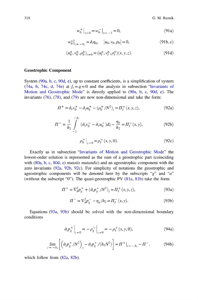
System (90a, b, c, 90d, e), up to constant coefficients, is a simplification of system
(74a, b, 74c, d, 74e) at f s = q = 0 and the analysis in subsection “Invariants of
Motion and Geostrophic Mode” is directly applied to (90a, b, c, 90d, e). The
invariants (76), (78), and (79) are now non-dimensional and take the form:
Π
+ = ∂ x v
+
0 − ∂ y u
+
0 − ðρ
+
0 ̸ N
2
Þ z = Π
+
I ðx, y, zÞ,
ð92aÞ
Π
− =
1
h 2
Z − h 1
− 1
ð∂ x v
−
0 − ∂ y u
−
0 Þdz −
η 0
h 2
= Π
−
I ðx, yÞ,
ð92bÞ
ρ
+
0
z = 0
= ρ
+
I ðx, y, 0Þ.
ð92cÞ
Exactly as in subsection “Invariants of Motion and Geostrophic Mode” the
lowest-order solution is represented as the sum of a geostrophic part (coinciding
with (80a, b, c, 80d, e) mutatis mutandis) and an ageostrophic component with the
zero invariants (92a, 92b, 92c). For simplicity of notations the geostrophic and
ageostrophic components will be denoted here by the subscripts “g” and “a”
(without the subscript “0”). The quasi-geostrophic PV (81a, 81b) take the form:
Π
+ = ∇
2
h p
+
g + ð∂ z p
+
g ̸ N
2
Þ z = Π
+
I ðx, y, zÞ,
ð93aÞ
Π
− = ∇
2
h p
−
g − η g ̸ h 2 = Π
−
I ðx, yÞ.
ð93bÞ
Equations (93a, 93b) should be solved with the non-dimensional boundary
conditions
∂ z p
+
g
z = 0
= − ρ
+
g
z = 0
= − ρ
+
I ðx, y, 0Þ,
ð94aÞ
lim
z → − h 1
∂ z p
+
g ̸ N
2
z
− ∂ z p
+
g ̸ ðh 2 N
2
Þ
!
= Π
+
j z = − h 1 − Π
− ,
ð94bÞ
which follow from (82a, 82b).
318
G. M. Reznik
+
0
z = 0
= w
−
0
z = − 1
= 0,
ð91aÞ
w
±
0
z = − h 1
= ∂ t η 0 , ½u 0 , v 0 , p 0 = 0,
ð91b; cÞ
ðu
±
0 , v
±
0 , ρ
±
0 Þ t = 0 = ðu
±
I , v
±
I , ρ
±
I Þðx, y, zÞ.
ð91dÞ
Geostrophic Component
System (90a, b, c, 90d, e), up to constant coefficients, is a simplification of system
(74a, b, 74c, d, 74e) at f s = q = 0 and the analysis in subsection “Invariants of
Motion and Geostrophic Mode” is directly applied to (90a, b, c, 90d, e). The
invariants (76), (78), and (79) are now non-dimensional and take the form:
Π
+ = ∂ x v
+
0 − ∂ y u
+
0 − ðρ
+
0 ̸ N
2
Þ z = Π
+
I ðx, y, zÞ,
ð92aÞ
Π
− =
1
h 2
Z − h 1
− 1
ð∂ x v
−
0 − ∂ y u
−
0 Þdz −
η 0
h 2
= Π
−
I ðx, yÞ,
ð92bÞ
ρ
+
0
z = 0
= ρ
+
I ðx, y, 0Þ.
ð92cÞ
Exactly as in subsection “Invariants of Motion and Geostrophic Mode” the
lowest-order solution is represented as the sum of a geostrophic part (coinciding
with (80a, b, c, 80d, e) mutatis mutandis) and an ageostrophic component with the
zero invariants (92a, 92b, 92c). For simplicity of notations the geostrophic and
ageostrophic components will be denoted here by the subscripts “g” and “a”
(without the subscript “0”). The quasi-geostrophic PV (81a, 81b) take the form:
Π
+ = ∇
2
h p
+
g + ð∂ z p
+
g ̸ N
2
Þ z = Π
+
I ðx, y, zÞ,
ð93aÞ
Π
− = ∇
2
h p
−
g − η g ̸ h 2 = Π
−
I ðx, yÞ.
ð93bÞ
Equations (93a, 93b) should be solved with the non-dimensional boundary
conditions
∂ z p
+
g
z = 0
= − ρ
+
g
z = 0
= − ρ
+
I ðx, y, 0Þ,
ð94aÞ
lim
z → − h 1
∂ z p
+
g ̸ N
2
z
− ∂ z p
+
g ̸ ðh 2 N
2
Þ
!
= Π
+
j z = − h 1 − Π
− ,
ð94bÞ
which follow from (82a, 82b).
318
G. M. Reznik