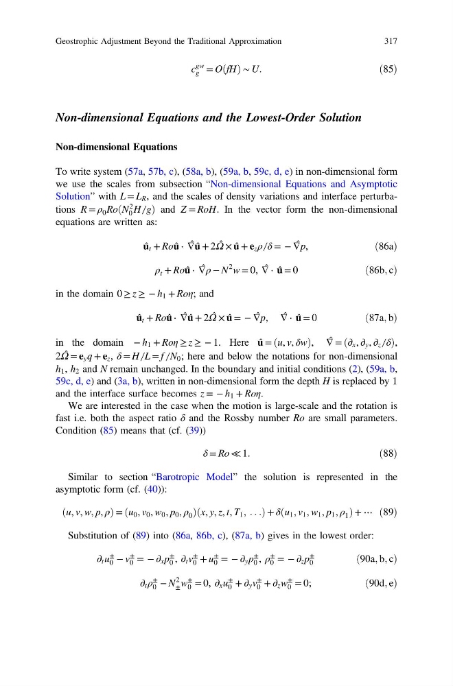
c
gw
g = OðfHÞ ∼ U.
ð85Þ
Non-dimensional Equations and the Lowest-Order Solution
Non-dimensional Equations
To write system (57a, 57b, c), (58a, b), (59a, b, 59c, d, e) in non-dimensional form
we use the scales from subsection “Non-dimensional Equations and Asymptotic
Solution” with L = L R , and the scales of density variations and interface perturbations R = ρ 0 RoðN
2
0 H ̸ gÞ and Z = RoH. In the vector form the non-dimensional
equations are written as:
û t + Roû ⋅ ∇ ̂ û + 2Ω ̂ × û + e z ρ ̸ δ = − ∇ ̂ p,
ð86aÞ
ρ t + Roû ⋅ ∇ ̂ ρ − N
2 w = 0, ∇ ̂ ⋅ û = 0
ð86b; cÞ
in the domain 0 ≥ z ≥ − h 1 + Roη; and
û t + Roû ⋅ ∇ ̂ û + 2Ω ̂ × û = − ∇ ̂ p, ∇ ̂ ⋅ û = 0
ð87a; bÞ
in the domain − h 1 + Roη ≥ z ≥ − 1. Here û = ðu, v, δwÞ, ∇ ̂ = ð∂ x , ∂ y , ∂ z ̸ δÞ,
2Ω ̂ = e y q + e z , δ = H ̸ L = f ̸ N 0 ; here and below the notations for non-dimensional
h 1 , h 2 and N remain unchanged. In the boundary and initial conditions (2), (59a, b,
59c, d, e) and (3a, b), written in non-dimensional form the depth H is replaced by 1
and the interface surface becomes z = − h 1 + Roη.
We are interested in the case when the motion is large-scale and the rotation is
fast i.e. both the aspect ratio δ and the Rossby number Ro are small parameters.
Condition (85) means that (cf. (39))
δ = Ro ≪ 1.
ð88Þ
Similar to section “Barotropic Model” the solution is represented in the
asymptotic form (cf. (40)):
ðu, v, w, p, ρÞ = ðu 0 , v 0 , w 0 , p 0 , ρ 0 Þðx, y, z, t, T 1 , . . .Þ + δðu 1 , v 1 , w 1 , p 1 , ρ 1 Þ + ⋯ ð89Þ
Substitution of (89) into (86a, 86b, c), (87a, b) gives in the lowest order:
∂ t u
±
0 − v
±
0 = − ∂ x p
±
0 , ∂ t v
±
0 + u
±
0 = − ∂ y p
±
0 , ρ
±
0 = − ∂ z p
±
0
ð90a; b; cÞ
∂ t ρ
±
0 − N
2
± w
±
0 = 0, ∂ x u
±
0 + ∂ y v
±
0 + ∂ z w
±
0 = 0;
ð90d; eÞ
Geostrophic Adjustment Beyond the Traditional Approximation
317