

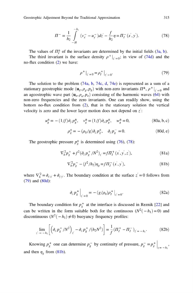
Π
− =
1
h 2
Z − h 1
− H
ðv
−
x ′ − u
−
y ′ Þdz
′
−
f
h 2
η = Π
−
I ðx
′ , y
′
Þ.
ð78Þ
The values of Π
±
I of the invariants are determined by the initial fields (3a, b).
The third invariant is the surface density ρ
+
j z ′ = 0 ; in view of (74d) and the
no-flux condition (2) we have:
ρ
+
j z ′ = 0 = ρ
+
I
z ′ = 0
.
ð79Þ
The solution to the problem (74a, b, 74c, d, 74e) is represented as a sum of a
stationary geostrophic mode ðu g , ρ g , p g Þ with non-zero invariants Π
± , ρ
+
j z ′ = 0 and
an ageostrophic wave part ðu a , ρ a , p a Þ consisting of the harmonic waves (64) with
non-zero frequencies and the zero invariants. One can readily show, using the
bottom no-flux condition from (2), that in the stationary solution the vertical
velocity is zero and the lower layer motion does not depend on z
′ :
u
±
g = − ð1 ̸ f Þ∂ y ′ p
±
g , v
±
g = ð1 ̸ f Þ∂ x ′ p
±
g , w
±
g = 0,
ð80a; b; cÞ
ρ
±
g = − ðρ 0 ̸ gÞ∂ z ′ p
±
g , ∂ z ′ p
−
g = 0.
ð80d; eÞ
The geostrophic pressure p
±
g is determined using (76), (78):
∇
′2
h p
+
g + f
2
ð∂ z ′ p
+
g ̸ N
2
Þ z ′ = f Π
+
I ðx
′ , y
′ , z
′
Þ,
ð81aÞ
∇
′2
h p
−
g − ðf
2
̸ h 2 Þη g = f Π
−
I ðx
′ , y
′
Þ,
ð81bÞ
where ∇
′2
h = ∂ x ′ x ′ + ∂ y ′ y ′ . The boundary condition at the surface z
′ = 0 follows from
(79) and (80d):
∂ z ′ p
+
g
z ′ = 0
= − ðg ̸ ρ 0 Þρ
+
I
z ′ = 0
.
ð82aÞ
The boundary condition for p
+
g at the interface is discussed in Reznik [22] and
can be written in the form suitable both for the continuous (N
2
ð − h 1 Þ = 0) and
discontinuous (N
2
ð − h 1 Þ ≠ 0) buoyancy frequency profiles:
lim
z ′ → − h 1
∂ z ′ p
+
g ̸ N
2
z ′
− ∂ z ′ p
+
g ̸ ðh 2 N
2
Þ
!
=
1
f
ðΠ
+
I − Π
−
I Þ z ′ = − h 1 .
ð82bÞ
Knowing p
+
g one can determine p
−
g by continuity of pressure, p
−
g = p
+
g
z = − h 1
,
and then η g from (81b).
Geostrophic Adjustment Beyond the Traditional Approximation
315
− =
1
h 2
Z − h 1
− H
ðv
−
x ′ − u
−
y ′ Þdz
′
−
f
h 2
η = Π
−
I ðx
′ , y
′
Þ.
ð78Þ
The values of Π
±
I of the invariants are determined by the initial fields (3a, b).
The third invariant is the surface density ρ
+
j z ′ = 0 ; in view of (74d) and the
no-flux condition (2) we have:
ρ
+
j z ′ = 0 = ρ
+
I
z ′ = 0
.
ð79Þ
The solution to the problem (74a, b, 74c, d, 74e) is represented as a sum of a
stationary geostrophic mode ðu g , ρ g , p g Þ with non-zero invariants Π
± , ρ
+
j z ′ = 0 and
an ageostrophic wave part ðu a , ρ a , p a Þ consisting of the harmonic waves (64) with
non-zero frequencies and the zero invariants. One can readily show, using the
bottom no-flux condition from (2), that in the stationary solution the vertical
velocity is zero and the lower layer motion does not depend on z
′ :
u
±
g = − ð1 ̸ f Þ∂ y ′ p
±
g , v
±
g = ð1 ̸ f Þ∂ x ′ p
±
g , w
±
g = 0,
ð80a; b; cÞ
ρ
±
g = − ðρ 0 ̸ gÞ∂ z ′ p
±
g , ∂ z ′ p
−
g = 0.
ð80d; eÞ
The geostrophic pressure p
±
g is determined using (76), (78):
∇
′2
h p
+
g + f
2
ð∂ z ′ p
+
g ̸ N
2
Þ z ′ = f Π
+
I ðx
′ , y
′ , z
′
Þ,
ð81aÞ
∇
′2
h p
−
g − ðf
2
̸ h 2 Þη g = f Π
−
I ðx
′ , y
′
Þ,
ð81bÞ
where ∇
′2
h = ∂ x ′ x ′ + ∂ y ′ y ′ . The boundary condition at the surface z
′ = 0 follows from
(79) and (80d):
∂ z ′ p
+
g
z ′ = 0
= − ðg ̸ ρ 0 Þρ
+
I
z ′ = 0
.
ð82aÞ
The boundary condition for p
+
g at the interface is discussed in Reznik [22] and
can be written in the form suitable both for the continuous (N
2
ð − h 1 Þ = 0) and
discontinuous (N
2
ð − h 1 Þ ≠ 0) buoyancy frequency profiles:
lim
z ′ → − h 1
∂ z ′ p
+
g ̸ N
2
z ′
− ∂ z ′ p
+
g ̸ ðh 2 N
2
Þ
!
=
1
f
ðΠ
+
I − Π
−
I Þ z ′ = − h 1 .
ð82bÞ
Knowing p
+
g one can determine p
−
g by continuity of pressure, p
−
g = p
+
g
z = − h 1
,
and then η g from (81b).
Geostrophic Adjustment Beyond the Traditional Approximation
315