

Slow Evolution
Under the TA, i.e. for q = 0, Eq. (44a) is substantially simplified, especially if the
QG streamfunction ψ is axisymmetric and, therefore, it does not depend on time as
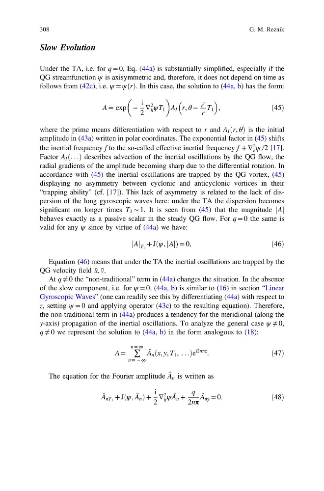
follows from (42c), i.e. ψ = ψðrÞ. In this case, the solution to (44a, b) has the form:
A = exp −
i
2
∇
2
h ψT 1
A I r, θ −
ψ ′
r
T 1
,
ð45Þ
where the prime means differentiation with respect to r and A I ðr, θÞ is the initial
amplitude in (43a) written in polar coordinates. The exponential factor in (45) shifts
the inertial frequency f to the so-called effective inertial frequency f + ∇
2
h ψ ̸ 2 [17].
Factor A I ð. . .Þ describes advection of the inertial oscillations by the QG flow, the
radial gradients of the amplitude becoming sharp due to the differential rotation. In
accordance with (45) the inertial oscillations are trapped by the QG vortex, (45)
displaying no asymmetry between cyclonic and anticyclonic vortices in their
“trapping ability” (cf. [17]). This lack of asymmetry is related to the lack of dispersion of the long gyroscopic waves here: under the TA the dispersion becomes
significant on longer times T 2 ∼ 1. It is seen from (45) that the magnitude A
j j
behaves exactly as a passive scalar in the steady QG flow. For q = 0 the same is
valid for any ψ since by virtue of (44a) we have:
A
j j T 1 + Jðψ, A
j jÞ= 0,
ð46Þ
Equation (46) means that under the TA the inertial oscillations are trapped by the
QG velocity field ū , v̄ .
At q ≠ 0 the “non-traditional” term in (44a) changes the situation. In the absence
of the slow component, i.e. for ψ = 0, (44a, b) is similar to (16) in section “Linear
Gyroscopic Waves” (one can readily see this by differentiating (44a) with respect to
z, setting ψ = 0 and applying operator (43c) to the resulting equation). Therefore,
the non-traditional term in (44a) produces a tendency for the meridional (along the
y-axis) propagation of the inertial oscillations. To analyze the general case ψ ≠ 0,
q ≠ 0 we represent the solution to (44a, b) in the form analogous to (18):
A = ∑
n = ∞
n = − ∞
A ̂ n ðx, y, T 1 , . . .Þe
i2nπz .
ð47Þ
The equation for the Fourier amplitude A ̂
n is written as
A ̂
nT 1 + Jðψ, A ̂
n Þ +
i
2
∇
2
h ψA ̂
n +
q
2nπ
A ̂
ny = 0.
ð48Þ
308
G. M. Reznik
Under the TA, i.e. for q = 0, Eq. (44a) is substantially simplified, especially if the
QG streamfunction ψ is axisymmetric and, therefore, it does not depend on time as
follows from (42c), i.e. ψ = ψðrÞ. In this case, the solution to (44a, b) has the form:
A = exp −
i
2
∇
2
h ψT 1
A I r, θ −
ψ ′
r
T 1
,
ð45Þ
where the prime means differentiation with respect to r and A I ðr, θÞ is the initial
amplitude in (43a) written in polar coordinates. The exponential factor in (45) shifts
the inertial frequency f to the so-called effective inertial frequency f + ∇
2
h ψ ̸ 2 [17].
Factor A I ð. . .Þ describes advection of the inertial oscillations by the QG flow, the
radial gradients of the amplitude becoming sharp due to the differential rotation. In
accordance with (45) the inertial oscillations are trapped by the QG vortex, (45)
displaying no asymmetry between cyclonic and anticyclonic vortices in their
“trapping ability” (cf. [17]). This lack of asymmetry is related to the lack of dispersion of the long gyroscopic waves here: under the TA the dispersion becomes
significant on longer times T 2 ∼ 1. It is seen from (45) that the magnitude A
j j
behaves exactly as a passive scalar in the steady QG flow. For q = 0 the same is
valid for any ψ since by virtue of (44a) we have:
A
j j T 1 + Jðψ, A
j jÞ= 0,
ð46Þ
Equation (46) means that under the TA the inertial oscillations are trapped by the
QG velocity field ū , v̄ .
At q ≠ 0 the “non-traditional” term in (44a) changes the situation. In the absence
of the slow component, i.e. for ψ = 0, (44a, b) is similar to (16) in section “Linear
Gyroscopic Waves” (one can readily see this by differentiating (44a) with respect to
z, setting ψ = 0 and applying operator (43c) to the resulting equation). Therefore,
the non-traditional term in (44a) produces a tendency for the meridional (along the
y-axis) propagation of the inertial oscillations. To analyze the general case ψ ≠ 0,
q ≠ 0 we represent the solution to (44a, b) in the form analogous to (18):
A = ∑
n = ∞
n = − ∞
A ̂ n ðx, y, T 1 , . . .Þe
i2nπz .
ð47Þ
The equation for the Fourier amplitude A ̂
n is written as
A ̂
nT 1 + Jðψ, A ̂
n Þ +
i
2
∇
2
h ψA ̂
n +
q
2nπ
A ̂
ny = 0.
ð48Þ
308
G. M. Reznik