

Ro = δ ≪ 1.
ð39Þ
Solution to the problem (38a, 38b, 38c, 38d), (2), (3a, b) is represented in the
form of multiple timescale asymptotic expansions analogous to (12):
ðu, v, w, pÞ = ðu 0 , v 0 , w 0 , p 0 Þðx, y, z, t, T 1 , . . .Þ + δðu 1 , v 1 , w 1 , p 1 Þ + . . . .
ð40Þ
Details of the calculation of successive terms in (40) can be found in Reznik
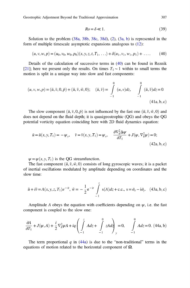
[21]; here we present only the results. On times T 1 ∼ 1 within to small terms the
motion is split in a unique way into slow and fast components:
ðu, v, w, pÞ = ðū , v̄ , 0, p̄ Þ + ðũ , ṽ , w̃ , 0Þ; ðū , v̄ Þ =
Z 0
− 1
ðu, vÞdz,
Z 0
− 1
ðũ , ṽ Þdz = 0.
ð41a; b; cÞ
The slow component ðū , v̄ , 0, p̄ Þ is not influenced by the fast one ðũ , ṽ , w̃ , 0Þ and
does not depend on the fluid depth; it is quasigeostrophic (QG) and obeys the QG
potential vorticity equation coinciding here with 2D fluid dynamics equation:
ū = ū ðx, y, T 1 Þ = − ψ y , v̄ = v̄ ðx, y, T 1 Þ = ψ x ,
∂∇
2
h Δψ
∂T 1
+ Jðψ, ∇
2
h ψÞ = 0;
ð42a; b; cÞ
ψ = ψðx, y, T 1 Þ is the QG streamfunction.
The fast component ðũ , ṽ , w̃ , 0Þ consists of long gyroscopic waves; it is a packet
of inertial oscillations modulated by amplitude depending on coordinates and the
slow time:
ũ + iṽ = Aðx, y, z, T 1 Þe
− it , w̃ = −
1
2
e
− it
Z z
− 1
sðAÞdz + c.c., s = ∂ x − i∂ y . ð43a; b; cÞ
Amplitude A obeys the equation with coefficients depending on ψ, i.e. the fast
component is coupled to the slow one:
∂A
∂T 1
+ Jðψ, AÞ +
i
2
∇
2
h ψA + iq
Z z
− 1
Adz +
Z 0
− 1
zAdz
0
@
1
A
y
= 0,
Z 0
− 1
Adz = 0. ð44a; bÞ
The term proportional q in (44a) is due to the “non-traditional” terms in the
equations of motion related to the horizontal component of Ω.
Geostrophic Adjustment Beyond the Traditional Approximation
307
ð39Þ
Solution to the problem (38a, 38b, 38c, 38d), (2), (3a, b) is represented in the
form of multiple timescale asymptotic expansions analogous to (12):
ðu, v, w, pÞ = ðu 0 , v 0 , w 0 , p 0 Þðx, y, z, t, T 1 , . . .Þ + δðu 1 , v 1 , w 1 , p 1 Þ + . . . .
ð40Þ
Details of the calculation of successive terms in (40) can be found in Reznik
[21]; here we present only the results. On times T 1 ∼ 1 within to small terms the
motion is split in a unique way into slow and fast components:
ðu, v, w, pÞ = ðū , v̄ , 0, p̄ Þ + ðũ , ṽ , w̃ , 0Þ; ðū , v̄ Þ =
Z 0
− 1
ðu, vÞdz,
Z 0
− 1
ðũ , ṽ Þdz = 0.
ð41a; b; cÞ
The slow component ðū , v̄ , 0, p̄ Þ is not influenced by the fast one ðũ , ṽ , w̃ , 0Þ and
does not depend on the fluid depth; it is quasigeostrophic (QG) and obeys the QG
potential vorticity equation coinciding here with 2D fluid dynamics equation:
ū = ū ðx, y, T 1 Þ = − ψ y , v̄ = v̄ ðx, y, T 1 Þ = ψ x ,
∂∇
2
h Δψ
∂T 1
+ Jðψ, ∇
2
h ψÞ = 0;
ð42a; b; cÞ
ψ = ψðx, y, T 1 Þ is the QG streamfunction.
The fast component ðũ , ṽ , w̃ , 0Þ consists of long gyroscopic waves; it is a packet
of inertial oscillations modulated by amplitude depending on coordinates and the
slow time:
ũ + iṽ = Aðx, y, z, T 1 Þe
− it , w̃ = −
1
2
e
− it
Z z
− 1
sðAÞdz + c.c., s = ∂ x − i∂ y . ð43a; b; cÞ
Amplitude A obeys the equation with coefficients depending on ψ, i.e. the fast
component is coupled to the slow one:
∂A
∂T 1
+ Jðψ, AÞ +
i
2
∇
2
h ψA + iq
Z z
− 1
Adz +
Z 0
− 1
zAdz
0
@
1
A
y
= 0,
Z 0
− 1
Adz = 0. ð44a; bÞ
The term proportional q in (44a) is due to the “non-traditional” terms in the
equations of motion related to the horizontal component of Ω.
Geostrophic Adjustment Beyond the Traditional Approximation
307