

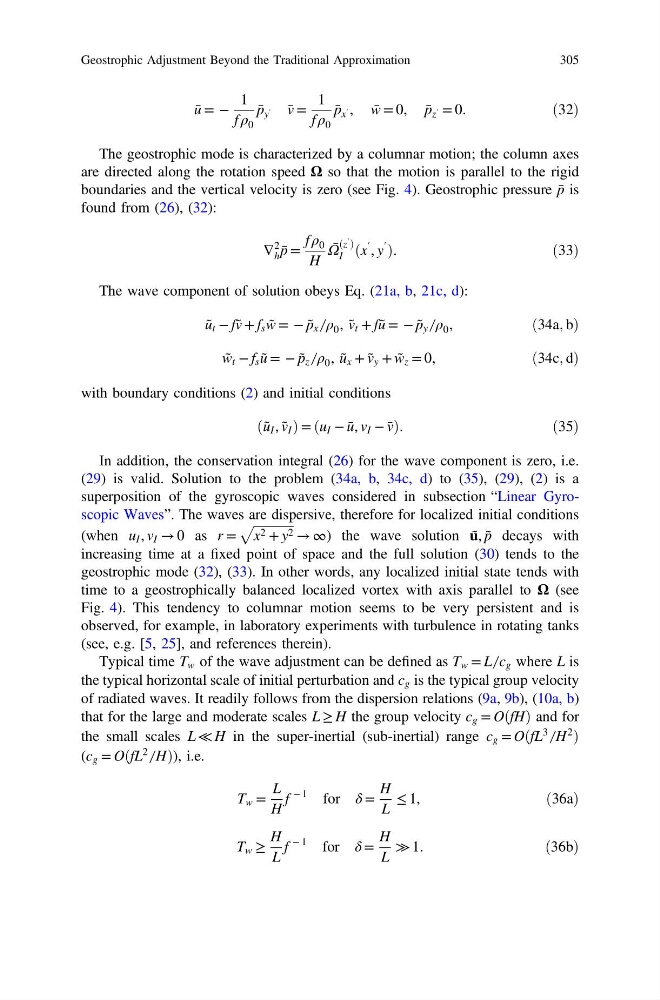
ū = −
1
f ρ 0
p̄ y ′ v̄ =
1
f ρ 0
p̄ x ′ , w̄ = 0, p̄ z ′ = 0.
ð32Þ
The geostrophic mode is characterized by a columnar motion; the column axes
are directed along the rotation speed Ω so that the motion is parallel to the rigid
boundaries and the vertical velocity is zero (see Fig. 4). Geostrophic pressure p̄ is
found from (26), (32):
∇
2
h p̄ =
f ρ 0
H
Ω ̄ ðz
′ Þ
I ðx
′ , y
′
Þ.
ð33Þ
The wave component of solution obeys Eq. (21a, b, 21c, d):
ũ t − fṽ + f s w̃ = − p̃ x ̸ ρ 0 , ṽ t + fũ = − p̃ y ̸ ρ 0 ,
ð34a; bÞ
w̃ t − f s ũ = − p̃ z ̸ ρ 0 , ũ x + ṽ y + w̃ z = 0,
ð34c; dÞ
with boundary conditions (2) and initial conditions
ðũ I , ṽ I Þ = ðu I − ū , v I − v̄ Þ.
ð35Þ
In addition, the conservation integral (26) for the wave component is zero, i.e.
(29) is valid. Solution to the problem (34a, b, 34c, d) to (35), (29), (2) is a
superposition of the gyroscopic waves considered in subsection “Linear Gyroscopic Waves”. The waves are dispersive, therefore for localized initial conditions
(when u I , v I → 0 as r =
ffiffiffiffiffiffiffiffiffiffiffiffiffi
x 2 + y 2
p
→ ∞) the wave solution ũ , p̃ decays with
increasing time at a fixed point of space and the full solution (30) tends to the
geostrophic mode (32), (33). In other words, any localized initial state tends with
time to a geostrophically balanced localized vortex with axis parallel to Ω (see
Fig. 4). This tendency to columnar motion seems to be very persistent and is
observed, for example, in laboratory experiments with turbulence in rotating tanks
(see, e.g. [5, 25], and references therein).
Typical time T w of the wave adjustment can be defined as T w = L ̸ c g where L is
the typical horizontal scale of initial perturbation and c g is the typical group velocity
of radiated waves. It readily follows from the dispersion relations (9a, 9b), (10a, b)
that for the large and moderate scales L ≥ H the group velocity c g = OðfHÞ and for
the small scales L ≪ H in the super-inertial (sub-inertial) range c g = OðfL
3
̸ H
2
Þ
(c g = OðfL
2
̸ HÞ), i.e.
T w =
L
H
f
− 1 for δ =
H
L
≤ 1,
ð36aÞ
T w ≥
H
L
f
− 1 for δ =
H
L
≫ 1.
ð36bÞ
Geostrophic Adjustment Beyond the Traditional Approximation
305
1
f ρ 0
p̄ y ′ v̄ =
1
f ρ 0
p̄ x ′ , w̄ = 0, p̄ z ′ = 0.
ð32Þ
The geostrophic mode is characterized by a columnar motion; the column axes
are directed along the rotation speed Ω so that the motion is parallel to the rigid
boundaries and the vertical velocity is zero (see Fig. 4). Geostrophic pressure p̄ is
found from (26), (32):
∇
2
h p̄ =
f ρ 0
H
Ω ̄ ðz
′ Þ
I ðx
′ , y
′
Þ.
ð33Þ
The wave component of solution obeys Eq. (21a, b, 21c, d):
ũ t − fṽ + f s w̃ = − p̃ x ̸ ρ 0 , ṽ t + fũ = − p̃ y ̸ ρ 0 ,
ð34a; bÞ
w̃ t − f s ũ = − p̃ z ̸ ρ 0 , ũ x + ṽ y + w̃ z = 0,
ð34c; dÞ
with boundary conditions (2) and initial conditions
ðũ I , ṽ I Þ = ðu I − ū , v I − v̄ Þ.
ð35Þ
In addition, the conservation integral (26) for the wave component is zero, i.e.
(29) is valid. Solution to the problem (34a, b, 34c, d) to (35), (29), (2) is a
superposition of the gyroscopic waves considered in subsection “Linear Gyroscopic Waves”. The waves are dispersive, therefore for localized initial conditions
(when u I , v I → 0 as r =
ffiffiffiffiffiffiffiffiffiffiffiffiffi
x 2 + y 2
p
→ ∞) the wave solution ũ , p̃ decays with
increasing time at a fixed point of space and the full solution (30) tends to the
geostrophic mode (32), (33). In other words, any localized initial state tends with
time to a geostrophically balanced localized vortex with axis parallel to Ω (see
Fig. 4). This tendency to columnar motion seems to be very persistent and is
observed, for example, in laboratory experiments with turbulence in rotating tanks
(see, e.g. [5, 25], and references therein).
Typical time T w of the wave adjustment can be defined as T w = L ̸ c g where L is
the typical horizontal scale of initial perturbation and c g is the typical group velocity
of radiated waves. It readily follows from the dispersion relations (9a, 9b), (10a, b)
that for the large and moderate scales L ≥ H the group velocity c g = OðfHÞ and for
the small scales L ≪ H in the super-inertial (sub-inertial) range c g = OðfL
3
̸ H
2
Þ
(c g = OðfL
2
̸ HÞ), i.e.
T w =
L
H
f
− 1 for δ =
H
L
≤ 1,
ð36aÞ
T w ≥
H
L
f
− 1 for δ =
H
L
≫ 1.
ð36bÞ
Geostrophic Adjustment Beyond the Traditional Approximation
305