

conservation law ∂ t h 1 + η
ð
Þ+ ∂ x h 1 + η
ð
ÞU
½
= 0, the relationship between the IIW
soliton amplitude A(x,t) and the velocity field at the surface Uðx, tÞ [12]:
Uðx, tÞ = c
Aðx, tÞ ̸ h 1
1 + Aðx, tÞ ̸ h 1
ð16Þ
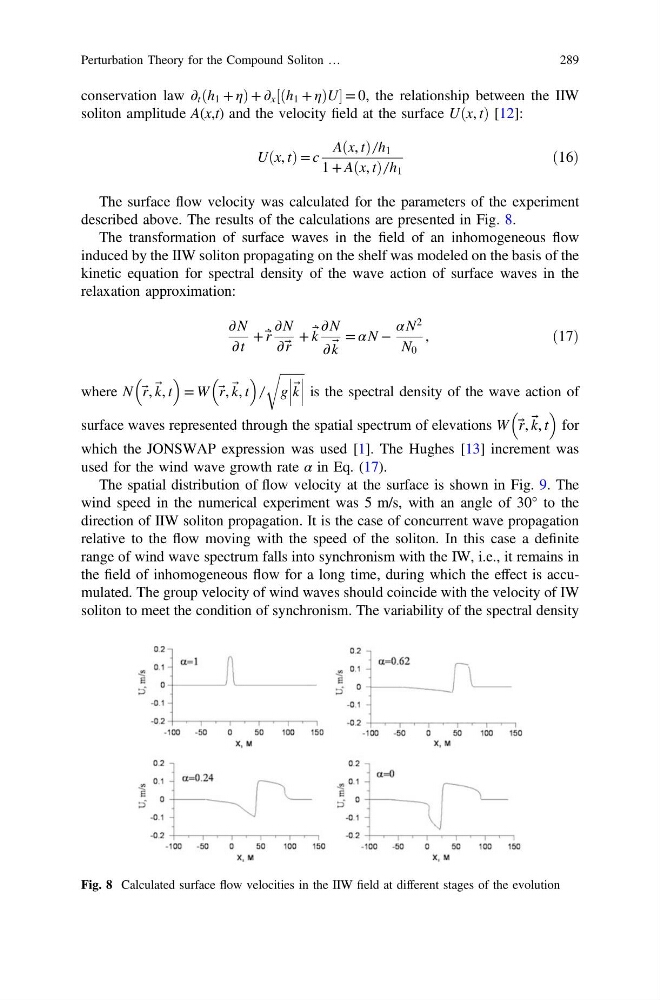
The surface flow velocity was calculated for the parameters of the experiment
described above. The results of the calculations are presented in Fig. 8.
The transformation of surface waves in the field of an inhomogeneous flow
induced by the IIW soliton propagating on the shelf was modeled on the basis of the
kinetic equation for spectral density of the wave action of surface waves in the
relaxation approximation:
∂ N
∂ t
+ r⃗ ̇ ∂ N
∂ r⃗
+ k ⃗ ̇ ∂ N
∂ k ⃗
= α N −
α N
2
N 0
,
ð17Þ
where N r⃗ , k ⃗
, t
= W r⃗ , k ⃗
, t
̸
ffiffiffiffiffiffiffiffi
g k ⃗
r
is the spectral density of the wave action of
surface waves represented through the spatial spectrum of elevations W r⃗ , k ⃗
, t
for
which the JONSWAP expression was used [1]. The Hughes [13] increment was
used for the wind wave growth rate α in Eq. (17).
The spatial distribution of flow velocity at the surface is shown in Fig. 9. The
wind speed in the numerical experiment was 5 m/s, with an angle of 30° to the
direction of IIW soliton propagation. It is the case of concurrent wave propagation
relative to the flow moving with the speed of the soliton. In this case a definite
range of wind wave spectrum falls into synchronism with the IW, i.e., it remains in
the field of inhomogeneous flow for a long time, during which the effect is accumulated. The group velocity of wind waves should coincide with the velocity of IW
soliton to meet the condition of synchronism. The variability of the spectral density
Fig. 8 Calculated surface flow velocities in the IIW field at different stages of the evolution
Perturbation Theory for the Compound Soliton …
289
ð
Þ+ ∂ x h 1 + η
ð
ÞU
½
= 0, the relationship between the IIW
soliton amplitude A(x,t) and the velocity field at the surface Uðx, tÞ [12]:
Uðx, tÞ = c
Aðx, tÞ ̸ h 1
1 + Aðx, tÞ ̸ h 1
ð16Þ
The surface flow velocity was calculated for the parameters of the experiment
described above. The results of the calculations are presented in Fig. 8.
The transformation of surface waves in the field of an inhomogeneous flow
induced by the IIW soliton propagating on the shelf was modeled on the basis of the
kinetic equation for spectral density of the wave action of surface waves in the
relaxation approximation:
∂ N
∂ t
+ r⃗ ̇ ∂ N
∂ r⃗
+ k ⃗ ̇ ∂ N
∂ k ⃗
= α N −
α N
2
N 0
,
ð17Þ
where N r⃗ , k ⃗
, t
= W r⃗ , k ⃗
, t
̸
ffiffiffiffiffiffiffiffi
g k ⃗
r
is the spectral density of the wave action of
surface waves represented through the spatial spectrum of elevations W r⃗ , k ⃗
, t
for
which the JONSWAP expression was used [1]. The Hughes [13] increment was
used for the wind wave growth rate α in Eq. (17).
The spatial distribution of flow velocity at the surface is shown in Fig. 9. The
wind speed in the numerical experiment was 5 m/s, with an angle of 30° to the
direction of IIW soliton propagation. It is the case of concurrent wave propagation
relative to the flow moving with the speed of the soliton. In this case a definite
range of wind wave spectrum falls into synchronism with the IW, i.e., it remains in
the field of inhomogeneous flow for a long time, during which the effect is accumulated. The group velocity of wind waves should coincide with the velocity of IW
soliton to meet the condition of synchronism. The variability of the spectral density
Fig. 8 Calculated surface flow velocities in the IIW field at different stages of the evolution
Perturbation Theory for the Compound Soliton …
289