

c =
ffiffiffiffiffiffiffiffiffiffiffiffiffiffiffiffiffiffiffiffiffiffiffi
gΔρ
ρ
h 1 h 2
h 1 + h 2
s
, β =
h 1 h 2
c 2 6
, α =
3
2
h 1 − h 2
ffiffiffiffiffiffiffiffiffiffiffiffiffi
2Δρgc
p
h 1 h 2
,
μ = −
3
16gΔρch
2
1 h
2
2
ðh
2
1 + h
2
2 + 6h 1 h 2 Þ, Φ =
ffiffiffiffiffiffiffiffiffiffiffiffiffi
2Δρgc
p
A, Δρ is the density jump
between the upper layer having thickness h 1 and is lower layer of thickness h 2 . In
the case typical of the shelf zone, the change in coefficients is due to the change in
depth and coefficients of the Gardner equation are functions of the variable τ =
R x
dx
c
that is a “ray” coordinate.
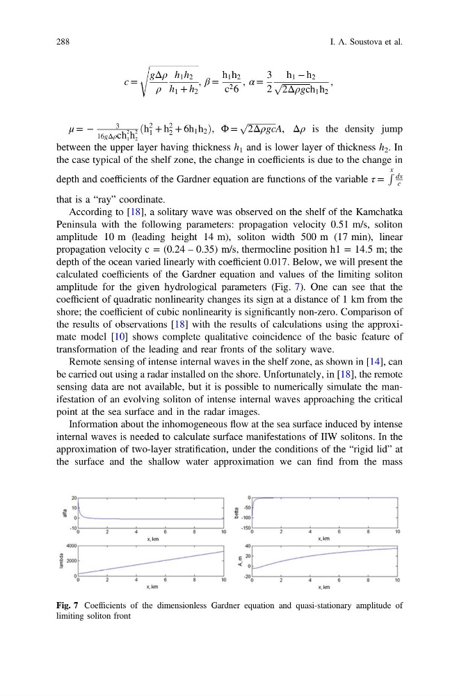
According to [18], a solitary wave was observed on the shelf of the Kamchatka
Peninsula with the following parameters: propagation velocity 0.51 m/s, soliton
amplitude 10 m (leading height 14 m), soliton width 500 m (17 min), linear
propagation velocity c = (0.24 – 0.35) m/s, thermocline position h1 = 14.5 m; the
depth of the ocean varied linearly with coefficient 0.017. Below, we will present the
calculated coefficients of the Gardner equation and values of the limiting soliton
amplitude for the given hydrological parameters (Fig. 7). One can see that the
coefficient of quadratic nonlinearity changes its sign at a distance of 1 km from the
shore; the coefficient of cubic nonlinearity is significantly non-zero. Comparison of
the results of observations [18] with the results of calculations using the approximate model [10] shows complete qualitative coincidence of the basic feature of
transformation of the leading and rear fronts of the solitary wave.
Remote sensing of intense internal waves in the shelf zone, as shown in [14], can
be carried out using a radar installed on the shore. Unfortunately, in [18], the remote
sensing data are not available, but it is possible to numerically simulate the manifestation of an evolving soliton of intense internal waves approaching the critical
point at the sea surface and in the radar images.
Information about the inhomogeneous flow at the sea surface induced by intense
internal waves is needed to calculate surface manifestations of IIW solitons. In the
approximation of two-layer stratification, under the conditions of the “rigid lid” at
the surface and the shallow water approximation we can find from the mass
Fig. 7 Coefficients of the dimensionless Gardner equation and quasi-stationary amplitude of
limiting soliton front
288
I. A. Soustova et al.
ffiffiffiffiffiffiffiffiffiffiffiffiffiffiffiffiffiffiffiffiffiffiffi
gΔρ
ρ
h 1 h 2
h 1 + h 2
s
, β =
h 1 h 2
c 2 6
, α =
3
2
h 1 − h 2
ffiffiffiffiffiffiffiffiffiffiffiffiffi
2Δρgc
p
h 1 h 2
,
μ = −
3
16gΔρch
2
1 h
2
2
ðh
2
1 + h
2
2 + 6h 1 h 2 Þ, Φ =
ffiffiffiffiffiffiffiffiffiffiffiffiffi
2Δρgc
p
A, Δρ is the density jump
between the upper layer having thickness h 1 and is lower layer of thickness h 2 . In
the case typical of the shelf zone, the change in coefficients is due to the change in
depth and coefficients of the Gardner equation are functions of the variable τ =
R x
dx
c
that is a “ray” coordinate.
According to [18], a solitary wave was observed on the shelf of the Kamchatka
Peninsula with the following parameters: propagation velocity 0.51 m/s, soliton
amplitude 10 m (leading height 14 m), soliton width 500 m (17 min), linear
propagation velocity c = (0.24 – 0.35) m/s, thermocline position h1 = 14.5 m; the
depth of the ocean varied linearly with coefficient 0.017. Below, we will present the
calculated coefficients of the Gardner equation and values of the limiting soliton
amplitude for the given hydrological parameters (Fig. 7). One can see that the
coefficient of quadratic nonlinearity changes its sign at a distance of 1 km from the
shore; the coefficient of cubic nonlinearity is significantly non-zero. Comparison of
the results of observations [18] with the results of calculations using the approximate model [10] shows complete qualitative coincidence of the basic feature of
transformation of the leading and rear fronts of the solitary wave.
Remote sensing of intense internal waves in the shelf zone, as shown in [14], can
be carried out using a radar installed on the shore. Unfortunately, in [18], the remote
sensing data are not available, but it is possible to numerically simulate the manifestation of an evolving soliton of intense internal waves approaching the critical
point at the sea surface and in the radar images.
Information about the inhomogeneous flow at the sea surface induced by intense
internal waves is needed to calculate surface manifestations of IIW solitons. In the
approximation of two-layer stratification, under the conditions of the “rigid lid” at
the surface and the shallow water approximation we can find from the mass
Fig. 7 Coefficients of the dimensionless Gardner equation and quasi-stationary amplitude of
limiting soliton front
288
I. A. Soustova et al.