

direction of its decay without changing their magnitude: the value of field Φ
+
c (t) is
equal to the value of the field near the front at a certain preceding moment of time
(t − τ). For a monotonically decreasing function αðtÞ, the field along the
quasi-soliton crest decreases monotonically from its decay to the front. Such a
character of the field persists up to the moment t = t cr , when α t cr
ð Þ= 0; hence,
Φ f (t cr ) = 0. The field near the decay Φ
+
c (t cr ) remains finite, and the field jump
becomes symmetric (Φ
+
c (t cr ) = − Φ
−
c (t cr )) and remains finite. while the size of the
quasi-soliton is LðtÞ = x f ðtÞ − x c ðtÞ due to the finiteness of the front and decay
speeds at all stages of the process. For decreasing function αðtÞ, the decay velocity
is always Φ
+
c Φ
+
c − α
À
Á ̸ 3 smaller than the front velocity, so that
LðtÞ = Lð0Þ + 1 ̸ 3
R t
0
Φ
+
c ðΦ
+
c − αÞdt increases monotonically in the 0 < t < t cr
interval, and the decay velocity in the neighborhood of α = 0 is always negative
(ẋ c ðt cr Þ = − ðΦ
+
c ðt cr ÞÞ
2 ̸ 3).
The regions near the quasi-soliton front and behind its decay remain problematic
for approximate description. As α → 0, the kink evolution at the front becomes
non-quasi-stationary due to its growing scale λ
− 1
m ≈ α
− 1
À
Á
. However, in view of the
relative smallness of the field values and of the size of the front-line region practically all the quasi-soliton crest is described correctly within the framework of the
proposed approach. In the region behind the decay the approximate approach gives
correct values of field Φ
−
c , but it does not adequately describe the field evolution as
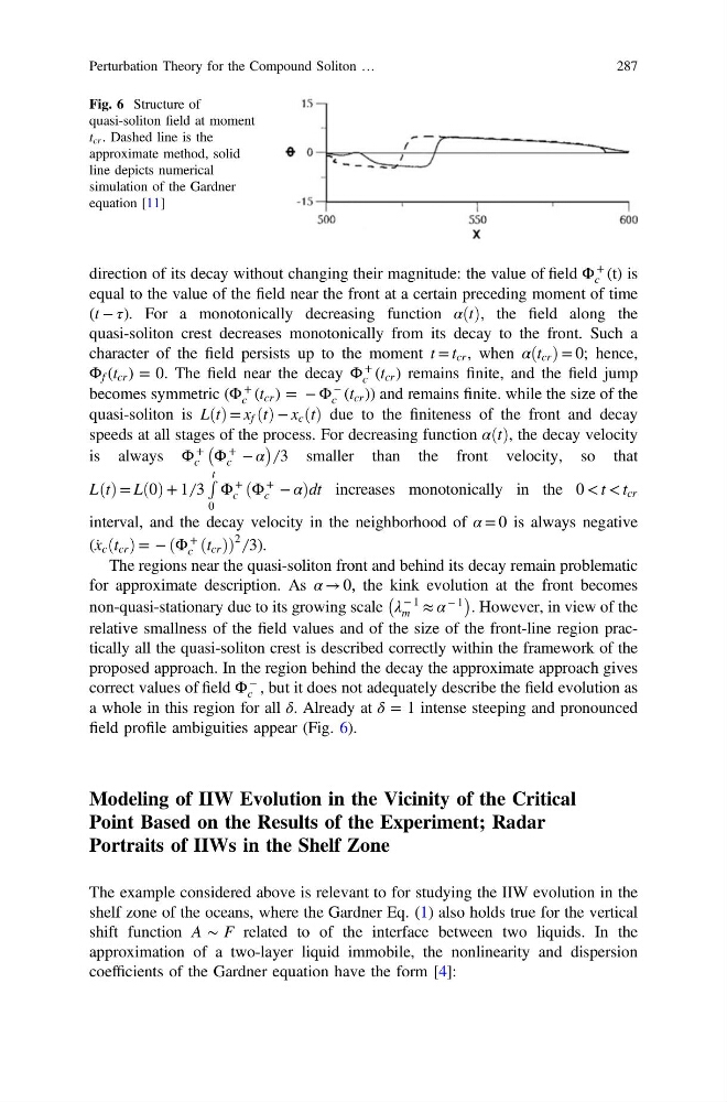
a whole in this region for all δ. Already at δ = 1 intense steeping and pronounced
field profile ambiguities appear (Fig. 6).
Modeling of IIW Evolution in the Vicinity of the Critical
Point Based on the Results of the Experiment; Radar
Portraits of IIWs in the Shelf Zone
The example considered above is relevant to for studying the IIW evolution in the
shelf zone of the oceans, where the Gardner Eq. (1) also holds true for the vertical
shift function A ∼ F related to of the interface between two liquids. In the
approximation of a two-layer liquid immobile, the nonlinearity and dispersion
coefficients of the Gardner equation have the form [4]:
Fig. 6 Structure of
quasi-soliton field at moment
t cr . Dashed line is the
approximate method, solid
line depicts numerical
simulation of the Gardner
equation [11]
Perturbation Theory for the Compound Soliton …
287
+
c (t) is
equal to the value of the field near the front at a certain preceding moment of time
(t − τ). For a monotonically decreasing function αðtÞ, the field along the
quasi-soliton crest decreases monotonically from its decay to the front. Such a
character of the field persists up to the moment t = t cr , when α t cr
ð Þ= 0; hence,
Φ f (t cr ) = 0. The field near the decay Φ
+
c (t cr ) remains finite, and the field jump
becomes symmetric (Φ
+
c (t cr ) = − Φ
−
c (t cr )) and remains finite. while the size of the
quasi-soliton is LðtÞ = x f ðtÞ − x c ðtÞ due to the finiteness of the front and decay
speeds at all stages of the process. For decreasing function αðtÞ, the decay velocity
is always Φ
+
c Φ
+
c − α
À
Á ̸ 3 smaller than the front velocity, so that
LðtÞ = Lð0Þ + 1 ̸ 3
R t
0
Φ
+
c ðΦ
+
c − αÞdt increases monotonically in the 0 < t < t cr
interval, and the decay velocity in the neighborhood of α = 0 is always negative
(ẋ c ðt cr Þ = − ðΦ
+
c ðt cr ÞÞ
2 ̸ 3).
The regions near the quasi-soliton front and behind its decay remain problematic
for approximate description. As α → 0, the kink evolution at the front becomes
non-quasi-stationary due to its growing scale λ
− 1
m ≈ α
− 1
À
Á
. However, in view of the
relative smallness of the field values and of the size of the front-line region practically all the quasi-soliton crest is described correctly within the framework of the
proposed approach. In the region behind the decay the approximate approach gives
correct values of field Φ
−
c , but it does not adequately describe the field evolution as
a whole in this region for all δ. Already at δ = 1 intense steeping and pronounced
field profile ambiguities appear (Fig. 6).
Modeling of IIW Evolution in the Vicinity of the Critical
Point Based on the Results of the Experiment; Radar
Portraits of IIWs in the Shelf Zone
The example considered above is relevant to for studying the IIW evolution in the
shelf zone of the oceans, where the Gardner Eq. (1) also holds true for the vertical
shift function A ∼ F related to of the interface between two liquids. In the
approximation of a two-layer liquid immobile, the nonlinearity and dispersion
coefficients of the Gardner equation have the form [4]:
Fig. 6 Structure of
quasi-soliton field at moment
t cr . Dashed line is the
approximate method, solid
line depicts numerical
simulation of the Gardner
equation [11]
Perturbation Theory for the Compound Soliton …
287