

defining the solitary wave evolution follows from the law of conservation of the
total soliton wave pulse
R
+ ∞
− ∞
Φ
2
s x, t
ð Þdx = P 0 = const; for Φ = 0 it has the following
form:
2r − th2r = P 0 α
− 2
μ
3
β
− 1
1
2
ð10Þ
The left-hand side of (10) as a function of r is increasing monotonically
throughout the 0 < r < + ∞ range, therefore the soliton scale increases without
restriction when the combination of the coefficients in the right-hand side of (10)
tends either to zero or to infinity. As the developed approach greatly relies on the
composite character of solitons, we will further address the
r → ∞, ð α
− 2
μ
3
β
− 1
1
2
Þ → ∞ limit. In a typical situation corresponding to this limit
in the case of IWs, the α(t) function has a point αðt cr Þ = 0 which in real conditions
corresponds to symmetric position of the thermocline. Such a problem was solved
numerically in [9] using linear function α t
ð Þ = 1 + εt. In this work, this problem is
solved analytically in a more general formulation.
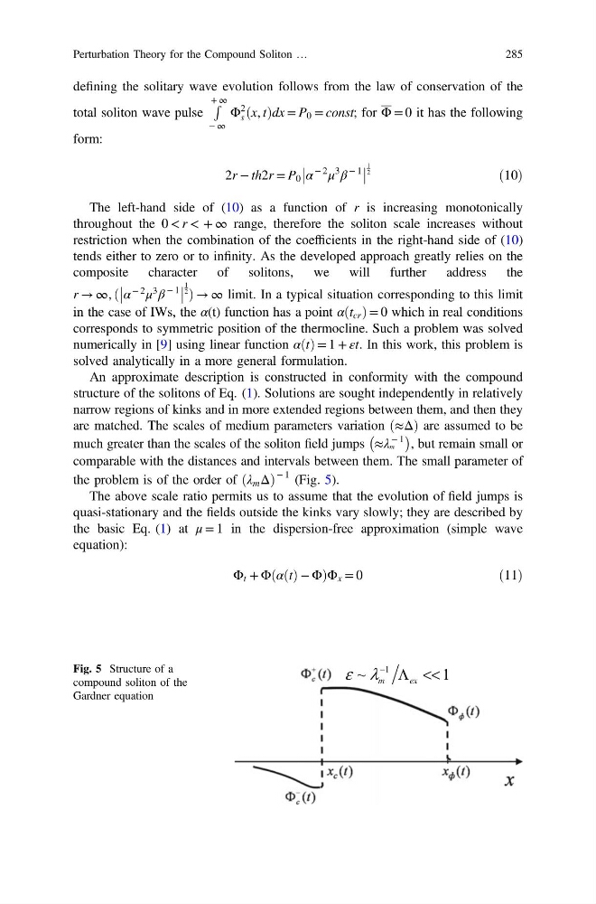
An approximate description is constructed in conformity with the compound
structure of the solitons of Eq. (1). Solutions are sought independently in relatively
narrow regions of kinks and in more extended regions between them, and then they
are matched. The scales of medium parameters variation ≈Δ
ð Þ are assumed to be
much greater than the scales of the soliton field jumps ≈λ
− 1
m
À
Á
, but remain small or
comparable with the distances and intervals between them. The small parameter of
the problem is of the order of ðλ m ΔÞ
− 1 (Fig. 5).
The above scale ratio permits us to assume that the evolution of field jumps is
quasi-stationary and the fields outside the kinks vary slowly; they are described by
the basic Eq. (1) at μ = 1 in the dispersion-free approximation (simple wave
equation):
Φ t + ΦðαðtÞ − ΦÞΦ x = 0
ð11Þ
1
~
1
m
e x
ε λ
−
Λ <<
Fig. 5 Structure of a
compound soliton of the
Gardner equation
Perturbation Theory for the Compound Soliton …
285
total soliton wave pulse
R
+ ∞
− ∞
Φ
2
s x, t
ð Þdx = P 0 = const; for Φ = 0 it has the following
form:
2r − th2r = P 0 α
− 2
μ
3
β
− 1
1
2
ð10Þ
The left-hand side of (10) as a function of r is increasing monotonically
throughout the 0 < r < + ∞ range, therefore the soliton scale increases without
restriction when the combination of the coefficients in the right-hand side of (10)
tends either to zero or to infinity. As the developed approach greatly relies on the
composite character of solitons, we will further address the
r → ∞, ð α
− 2
μ
3
β
− 1
1
2
Þ → ∞ limit. In a typical situation corresponding to this limit
in the case of IWs, the α(t) function has a point αðt cr Þ = 0 which in real conditions
corresponds to symmetric position of the thermocline. Such a problem was solved
numerically in [9] using linear function α t
ð Þ = 1 + εt. In this work, this problem is
solved analytically in a more general formulation.
An approximate description is constructed in conformity with the compound
structure of the solitons of Eq. (1). Solutions are sought independently in relatively
narrow regions of kinks and in more extended regions between them, and then they
are matched. The scales of medium parameters variation ≈Δ
ð Þ are assumed to be
much greater than the scales of the soliton field jumps ≈λ
− 1
m
À
Á
, but remain small or
comparable with the distances and intervals between them. The small parameter of
the problem is of the order of ðλ m ΔÞ
− 1 (Fig. 5).
The above scale ratio permits us to assume that the evolution of field jumps is
quasi-stationary and the fields outside the kinks vary slowly; they are described by
the basic Eq. (1) at μ = 1 in the dispersion-free approximation (simple wave
equation):
Φ t + ΦðαðtÞ − ΦÞΦ x = 0
ð11Þ
1
~
1
m
e x
ε λ
−
Λ <<
Fig. 5 Structure of a
compound soliton of the
Gardner equation
Perturbation Theory for the Compound Soliton …
285