

Simulation of Standing and Propagating Sea Waves . . .
275
∙ The order of frequencies in Fourier transforms is different and clFFT library
requires reordering the result of (24) whereas GSL does not.
∙ Discontinuity at (x, y) = (0, 0) of velocity potential field grid is handled automatically by clFFT library, whereas GSL library produce skewed values at this point.
For GSL library an additional interpolation from neighbouring points was used to
smooth velocity potential field at these points. We have not spotted other differences
in FFT implementations that have impact on the overall performance.
In the course of the numerical experiments we have measured how much time
each solver’s implementation spends in each computation stage to explain how efficient data copying between host and device is in OpenCL implementation, and how
one implementation corresponds to the other in terms of performance.
Results
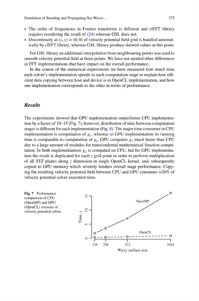
The experiments showed that GPU implementation outperforms CPU implementation by a factor of 10–15 (Fig. 7), however, distribution of time between computation
stages is different for each implementation (Fig. 8). The major time consumer in CPU
implementation is computation of g 1 , whereas in GPU implementation its running
time is comparable to computation of g 2 . GPU computes g 1 much faster than CPU
due to a large amount of modules for transcendental mathematical function computation. In both implementations g 2 is computed on CPU, but for GPU implementation the result is duplicated for each z grid point in order to perform multiplication
of all XYZ planes along z dimension in single OpenCL kernel, and, subsequently
copied to GPU memory which severely hinders overall stage performance. Copying the resulting velocity potential field between CPU and GPU consumes ≈20% of
velocity potential solver execution time.
Fig. 7 Performance
comparison of CPU
(OpenMP) and GPU
(OpenCL) versions of
velocity potential solver
128
256
512
1024
0
5
1 0
1 5
Wavy surface size
Time, s
OpenMP
OpenCL
275
∙ The order of frequencies in Fourier transforms is different and clFFT library
requires reordering the result of (24) whereas GSL does not.
∙ Discontinuity at (x, y) = (0, 0) of velocity potential field grid is handled automatically by clFFT library, whereas GSL library produce skewed values at this point.
For GSL library an additional interpolation from neighbouring points was used to
smooth velocity potential field at these points. We have not spotted other differences
in FFT implementations that have impact on the overall performance.
In the course of the numerical experiments we have measured how much time
each solver’s implementation spends in each computation stage to explain how efficient data copying between host and device is in OpenCL implementation, and how
one implementation corresponds to the other in terms of performance.
Results
The experiments showed that GPU implementation outperforms CPU implementation by a factor of 10–15 (Fig. 7), however, distribution of time between computation
stages is different for each implementation (Fig. 8). The major time consumer in CPU
implementation is computation of g 1 , whereas in GPU implementation its running
time is comparable to computation of g 2 . GPU computes g 1 much faster than CPU
due to a large amount of modules for transcendental mathematical function computation. In both implementations g 2 is computed on CPU, but for GPU implementation the result is duplicated for each z grid point in order to perform multiplication
of all XYZ planes along z dimension in single OpenCL kernel, and, subsequently
copied to GPU memory which severely hinders overall stage performance. Copying the resulting velocity potential field between CPU and GPU consumes ≈20% of
velocity potential solver execution time.
Fig. 7 Performance
comparison of CPU
(OpenMP) and GPU
(OpenCL) versions of
velocity potential solver
128
256
512
1024
0
5
1 0
1 5
Wavy surface size
Time, s
OpenMP
OpenCL