

274
I. Gankevich and A. Degtyarev
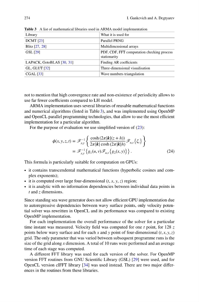
Table 3 A list of mathematical libraries used in ARMA model implementation
Library
What it is used for
DCMT [23]
Parallel PRNG
Blitz [27, 28]
Multidimensional arrays
GSL [29]
PDF, CDF, FFT computation checking process
stationarity
LAPACK, GotoBLAS [30, 31]
Finding AR coefficients
GL, GLUT [32]
Three-dimensional visualisation
CGAL [33]
Wave numbers triangulation
not to mention that high convergence rate and non-existence of periodicity allows to
use far fewer coefficients compared to LH model.
ARMA implementation uses several libraries of reusable mathematical functions
and numerical algorithms (listed in Table 3), and was implemented using OpenMP
and OpenCL parallel programming technologies, that allow to use the most efficient
implementation for a particular algorithm.
For the purpose of evaluation we use simplified version of (23):
í µí¼(x, y, z, t) = F
−1
x,y
{ cosh (2í µí¼|k|(z + h))
2í µí¼|k| cosh (2í µí¼|k|h)
F u,v
{ í µí¼ t
}
}
= F
−1
x,y
{
g 1 (u, v)F u,v
{
g 2 (x, y)
}} .
(24)
This formula is particularly suitable for computation on GPUs:
∙ it contains transcendental mathematical functions (hyperbolic cosines and complex exponents);
∙ it is computed over large four-dimensional (t, x, y, z) region;
∙ it is analytic with no information dependencies between individual data points in
t and z dimensions.
Since standing sea wave generator does not allow efficient GPU implementation due
to autoregressive dependencies between wavy surface points, only velocity potential solver was rewritten in OpenCL and its performance was compared to existing
OpenMP implementation.
For each implementation the overall performance of the solver for a particular
time instant was measured. Velocity field was computed for one t point, for 128 z
points below wavy surface and for each x and y point of four-dimensional (t, x, y, z)
grid. The only parameter that was varied between subsequent programme runs is the
size of the grid along x dimension. A total of 10 runs were performed and an average
time of each stage was computed.
A different FFT library was used for each version of the solver. For OpenMP
version FFT routines from GNU Scientific Library (GSL) [29] were used, and for
OpenCL version clFFT library [34] was used instead. There are two major differences in the routines from these libraries.
I. Gankevich and A. Degtyarev
Table 3 A list of mathematical libraries used in ARMA model implementation
Library
What it is used for
DCMT [23]
Parallel PRNG
Blitz [27, 28]
Multidimensional arrays
GSL [29]
PDF, CDF, FFT computation checking process
stationarity
LAPACK, GotoBLAS [30, 31]
Finding AR coefficients
GL, GLUT [32]
Three-dimensional visualisation
CGAL [33]
Wave numbers triangulation
not to mention that high convergence rate and non-existence of periodicity allows to
use far fewer coefficients compared to LH model.
ARMA implementation uses several libraries of reusable mathematical functions
and numerical algorithms (listed in Table 3), and was implemented using OpenMP
and OpenCL parallel programming technologies, that allow to use the most efficient
implementation for a particular algorithm.
For the purpose of evaluation we use simplified version of (23):
í µí¼(x, y, z, t) = F
−1
x,y
{ cosh (2í µí¼|k|(z + h))
2í µí¼|k| cosh (2í µí¼|k|h)
F u,v
{ í µí¼ t
}
}
= F
−1
x,y
{
g 1 (u, v)F u,v
{
g 2 (x, y)
}} .
(24)
This formula is particularly suitable for computation on GPUs:
∙ it contains transcendental mathematical functions (hyperbolic cosines and complex exponents);
∙ it is computed over large four-dimensional (t, x, y, z) region;
∙ it is analytic with no information dependencies between individual data points in
t and z dimensions.
Since standing sea wave generator does not allow efficient GPU implementation due
to autoregressive dependencies between wavy surface points, only velocity potential solver was rewritten in OpenCL and its performance was compared to existing
OpenMP implementation.
For each implementation the overall performance of the solver for a particular
time instant was measured. Velocity field was computed for one t point, for 128 z
points below wavy surface and for each x and y point of four-dimensional (t, x, y, z)
grid. The only parameter that was varied between subsequent programme runs is the
size of the grid along x dimension. A total of 10 runs were performed and an average
time of each stage was computed.
A different FFT library was used for each version of the solver. For OpenMP
version FFT routines from GNU Scientific Library (GSL) [29] were used, and for
OpenCL version clFFT library [34] was used instead. There are two major differences in the routines from these libraries.