

Simulation of Standing and Propagating Sea Waves . . .
273
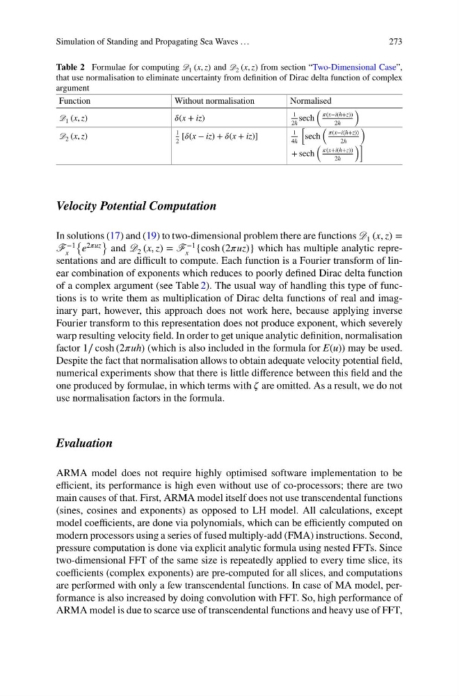
Table 2 Formulae for computing D 1 (x, z) and D 2 (x, z) from section “Two-Dimensional Case”,
that use normalisation to eliminate uncertainty from definition of Dirac delta function of complex
argument
Function
Without normalisation
Normalised
D 1 (x, z)
í µí»¿(x + iz)
1
2h
sech
( í µí¼(x−i(h+z))
2h
)
D 2 (x, z)
1
2
[í µí»¿(x − iz) + í µí»¿(x + iz)]
1
4h
[
sech
( í µí¼(x−i(h+z))
2h
)
+ sech
( í µí¼(x+i(h+z))
2h
)]
Velocity Potential Computation
In solutions (17) and (19) to two-dimensional problem there are functions D 1 (x, z) =
F
−1
x
{
e
2í µí¼uz
}
and D 2 (x, z) = F
−1
x {cosh (2í µí¼uz)} which has multiple analytic representations and are difficult to compute. Each function is a Fourier transform of linear combination of exponents which reduces to poorly defined Dirac delta function
of a complex argument (see Table 2). The usual way of handling this type of functions is to write them as multiplication of Dirac delta functions of real and imaginary part, however, this approach does not work here, because applying inverse
Fourier transform to this representation does not produce exponent, which severely
warp resulting velocity field. In order to get unique analytic definition, normalisation
factor 1∕ cosh (2í µí¼uh) (which is also included in the formula for E(u)) may be used.
Despite the fact that normalisation allows to obtain adequate velocity potential field,
numerical experiments show that there is little difference between this field and the
one produced by formulae, in which terms with í µí¼ are omitted. As a result, we do not
use normalisation factors in the formula.
Evaluation
ARMA model does not require highly optimised software implementation to be
efficient, its performance is high even without use of co-processors; there are two
main causes of that. First, ARMA model itself does not use transcendental functions
(sines, cosines and exponents) as opposed to LH model. All calculations, except
model coefficients, are done via polynomials, which can be efficiently computed on
modern processors using a series of fused multiply-add (FMA) instructions. Second,
pressure computation is done via explicit analytic formula using nested FFTs. Since
two-dimensional FFT of the same size is repeatedly applied to every time slice, its
coefficients (complex exponents) are pre-computed for all slices, and computations
are performed with only a few transcendental functions. In case of MA model, performance is also increased by doing convolution with FFT. So, high performance of
ARMA model is due to scarce use of transcendental functions and heavy use of FFT,
273
Table 2 Formulae for computing D 1 (x, z) and D 2 (x, z) from section “Two-Dimensional Case”,
that use normalisation to eliminate uncertainty from definition of Dirac delta function of complex
argument
Function
Without normalisation
Normalised
D 1 (x, z)
í µí»¿(x + iz)
1
2h
sech
( í µí¼(x−i(h+z))
2h
)
D 2 (x, z)
1
2
[í µí»¿(x − iz) + í µí»¿(x + iz)]
1
4h
[
sech
( í µí¼(x−i(h+z))
2h
)
+ sech
( í µí¼(x+i(h+z))
2h
)]
Velocity Potential Computation
In solutions (17) and (19) to two-dimensional problem there are functions D 1 (x, z) =
F
−1
x
{
e
2í µí¼uz
}
and D 2 (x, z) = F
−1
x {cosh (2í µí¼uz)} which has multiple analytic representations and are difficult to compute. Each function is a Fourier transform of linear combination of exponents which reduces to poorly defined Dirac delta function
of a complex argument (see Table 2). The usual way of handling this type of functions is to write them as multiplication of Dirac delta functions of real and imaginary part, however, this approach does not work here, because applying inverse
Fourier transform to this representation does not produce exponent, which severely
warp resulting velocity field. In order to get unique analytic definition, normalisation
factor 1∕ cosh (2í µí¼uh) (which is also included in the formula for E(u)) may be used.
Despite the fact that normalisation allows to obtain adequate velocity potential field,
numerical experiments show that there is little difference between this field and the
one produced by formulae, in which terms with í µí¼ are omitted. As a result, we do not
use normalisation factors in the formula.
Evaluation
ARMA model does not require highly optimised software implementation to be
efficient, its performance is high even without use of co-processors; there are two
main causes of that. First, ARMA model itself does not use transcendental functions
(sines, cosines and exponents) as opposed to LH model. All calculations, except
model coefficients, are done via polynomials, which can be efficiently computed on
modern processors using a series of fused multiply-add (FMA) instructions. Second,
pressure computation is done via explicit analytic formula using nested FFTs. Since
two-dimensional FFT of the same size is repeatedly applied to every time slice, its
coefficients (complex exponents) are pre-computed for all slices, and computations
are performed with only a few transcendental functions. In case of MA model, performance is also increased by doing convolution with FFT. So, high performance of
ARMA model is due to scarce use of transcendental functions and heavy use of FFT,