

Abyssal Mixing in the Laboratory
229
Figure 4 reveals the onset of TRI in the attractor. The numerical simulations clearly
emphasize the importance of boundary layers close to the walls, and thus the importance of the three-dimensionality to recover experimental laboratory results quantitatively, nevertheless 2D simulations are fully sufficient for qualitative agreement.
We checked [7, 16], that the temporal and spatial resonance conditions of TRI are
satisfied experimentally and numerically.
Comparison
We have carefully compared the results obtained experimentally and numerically.
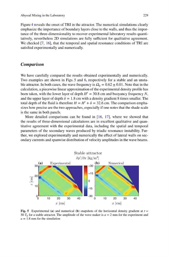
Two examples are shown in Figs. 5 and 6, respectively for a stable and an unstable attractor. In both cases, the wave frequency is í µí»º 0 = 0.62 ± 0.01. Note that in the
calculation, a piecewise linear approximation of the experimental density profile has
been taken, with the lower layer of depth H ′ = 30.8 cm and buoyancy frequency N,
and the upper layer of depth í µí»¿ = 1.8 cm with a density gradient 8 times smaller. The
total depth of the fluid is therefore H = H ′ + í µí»¿ = 32.6 cm. The comparison emphasizes how precise are the two approaches, especially if one notes that the shade scale
is the same in both panels.
More detailed comparisons can be found in [16, 17], where we showed that
the results of three-dimensional calculations are in excellent qualitative and quantitative agreement with the experimental data, including the spatial and temporal
parameters of the secondary waves produced by triadic resonance instability. Further, we explored experimentally and numerically the effect of lateral walls on secondary currents and spanwise distribution of velocity amplitudes in the wave beams.
0
10
20
30
-30
-15
0
+15
+30
0
10
20
30
40
0
10
20
30
40
(a)
(b)
Fig. 5 Experimental (a) and numerical (b) snapshots of the horizontal density gradient at t =
50 T 0 for a stable attractor. The amplitude of the wave maker is a = 2 mm for the experiment and
a = 1.8 mm for the simulation
229
Figure 4 reveals the onset of TRI in the attractor. The numerical simulations clearly
emphasize the importance of boundary layers close to the walls, and thus the importance of the three-dimensionality to recover experimental laboratory results quantitatively, nevertheless 2D simulations are fully sufficient for qualitative agreement.
We checked [7, 16], that the temporal and spatial resonance conditions of TRI are
satisfied experimentally and numerically.
Comparison
We have carefully compared the results obtained experimentally and numerically.
Two examples are shown in Figs. 5 and 6, respectively for a stable and an unstable attractor. In both cases, the wave frequency is í µí»º 0 = 0.62 ± 0.01. Note that in the
calculation, a piecewise linear approximation of the experimental density profile has
been taken, with the lower layer of depth H ′ = 30.8 cm and buoyancy frequency N,
and the upper layer of depth í µí»¿ = 1.8 cm with a density gradient 8 times smaller. The
total depth of the fluid is therefore H = H ′ + í µí»¿ = 32.6 cm. The comparison emphasizes how precise are the two approaches, especially if one notes that the shade scale
is the same in both panels.
More detailed comparisons can be found in [16, 17], where we showed that
the results of three-dimensional calculations are in excellent qualitative and quantitative agreement with the experimental data, including the spatial and temporal
parameters of the secondary waves produced by triadic resonance instability. Further, we explored experimentally and numerically the effect of lateral walls on secondary currents and spanwise distribution of velocity amplitudes in the wave beams.
0
10
20
30
-30
-15
0
+15
+30
0
10
20
30
40
0
10
20
30
40
(a)
(b)
Fig. 5 Experimental (a) and numerical (b) snapshots of the horizontal density gradient at t =
50 T 0 for a stable attractor. The amplitude of the wave maker is a = 2 mm for the experiment and
a = 1.8 mm for the simulation