

Large Internal Solitary Waves in Shallow Waters
105
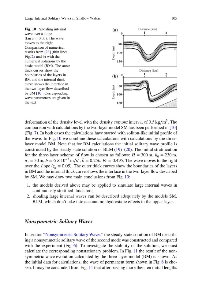
Fig. 10 Shoaling internal
wave over a slope
(tan í µí»¼ = 0.05). The wave
moves to the right.
Comparison of numerical
results from [28] (thin lines,
Fig. 2a and b) with the
numerical solutions by the
basic model (BM). The outer
thick curves show the
boundaries of the layers in
BM and the internal thick
curve shows the interface in
the two-layer flow described
by SM [10]. Corresponding
wave parameters are given in
the text
deformation of the density level with the density contour interval of 0.5 kg∕m
3 . The
comparison with calculations by the two-layer model SM has been performed in [10]
(Fig. 7). In both cases the calculations have started with soliton-like initial profile of
the wave. In Fig. 10 we combine these calculations with calculations by the threelayer model BM. Note that for BM calculations the initial solitary wave profile is
constructed by the steady-state solution of BLM (19)–(20). The initial stratification
for the three-layer scheme of flow is chosen as follows: H = 300 m, h 0 = 230 m,
í µí¼ 0 = 30 m, b = 6 × 10
−2
m∕s
2 , ̄
b = 0.25b, Fr = 0.495. The wave moves to the right
over the slope (z x ≡ 0.05). The outer thick curves show the boundaries of the layers
in BM and the internal thick curve shows the interface in the two-layer flow described
by SM. We may draw two main conclusions from Fig. 10:
1. the models derived above may be applied to simulate large internal waves in
continuously stratified fluids too;
2. shoaling large internal waves can be described adequately by the models SM,
BLM, which don’t take into account nonhydrostatic effects in the upper layer.
Nonsymmetric Solitary Waves
In section “Nonsymmetric Solitary Waves” the steady-state solution of BM describing a nonsymmetric solitary wave of the second mode was constructed and compared
with the experiment (Fig. 6). To investigate the stability of the solution, we must
calculate the corresponding nonstationary problem. In Fig. 11 the result of the nonsymmetric wave evolution calculated by the three-layer model (BM) is shown. As
the initial data for calculations, the wave of permanent form shown in Fig. 6 is chosen. It may be concluded from Fig. 11 that after passing more then ten initial lengths
105
Fig. 10 Shoaling internal
wave over a slope
(tan í µí»¼ = 0.05). The wave
moves to the right.
Comparison of numerical
results from [28] (thin lines,
Fig. 2a and b) with the
numerical solutions by the
basic model (BM). The outer
thick curves show the
boundaries of the layers in
BM and the internal thick
curve shows the interface in
the two-layer flow described
by SM [10]. Corresponding
wave parameters are given in
the text
deformation of the density level with the density contour interval of 0.5 kg∕m
3 . The
comparison with calculations by the two-layer model SM has been performed in [10]
(Fig. 7). In both cases the calculations have started with soliton-like initial profile of
the wave. In Fig. 10 we combine these calculations with calculations by the threelayer model BM. Note that for BM calculations the initial solitary wave profile is
constructed by the steady-state solution of BLM (19)–(20). The initial stratification
for the three-layer scheme of flow is chosen as follows: H = 300 m, h 0 = 230 m,
í µí¼ 0 = 30 m, b = 6 × 10
−2
m∕s
2 , ̄
b = 0.25b, Fr = 0.495. The wave moves to the right
over the slope (z x ≡ 0.05). The outer thick curves show the boundaries of the layers
in BM and the internal thick curve shows the interface in the two-layer flow described
by SM. We may draw two main conclusions from Fig. 10:
1. the models derived above may be applied to simulate large internal waves in
continuously stratified fluids too;
2. shoaling large internal waves can be described adequately by the models SM,
BLM, which don’t take into account nonhydrostatic effects in the upper layer.
Nonsymmetric Solitary Waves
In section “Nonsymmetric Solitary Waves” the steady-state solution of BM describing a nonsymmetric solitary wave of the second mode was constructed and compared
with the experiment (Fig. 6). To investigate the stability of the solution, we must
calculate the corresponding nonstationary problem. In Fig. 11 the result of the nonsymmetric wave evolution calculated by the three-layer model (BM) is shown. As
the initial data for calculations, the wave of permanent form shown in Fig. 6 is chosen. It may be concluded from Fig. 11 that after passing more then ten initial lengths