

104
V. Liapidevskii and N. Gavrilov
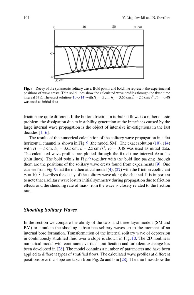
Fig. 9 Decay of the symmetric solitary wave. Bold points and bold line represent the experimental
positions of wave crests. Thin solid lines show the calculated wave profiles through the fixed time
interval (4 s). The exact solution (10), (14) with H 1 = 5 cm, h 0 = 3.65 cm, ̄
b = 2.5 cm∕s
2 , Fr = 0.48
was used as initial data
friction are quite different. If the bottom friction in turbulent flows is a rather classic
problem, the dissipation due to instability generation at the interfaces caused by the
large internal wave propagation is the object of intensive investigations in the last
decades [1, 6].
The results of the numerical calculation of the solitary wave propagation in a flat
horizontal channel is shown in Fig. 9 (the model SM). The exact solution (10), (14)
with H 1 = 5 cm, h 0 = 3.65 cm, ̄
b = 2.5 cm∕s
2 , Fr = 0.48 was used as initial data.
The calculated wave profiles are plotted through the fixed time interval Δt = 4 s
(thin lines). The bold points in Fig. 9 together with the bold line passing through
them are the positions of the solitary wave crests found from experiments [9]. One
can see from Fig. 9 that the mathematical model (4), (27) with the friction coefficient
c i = 10
−2 describes the decay of the solitary wave along the channel. It is important
to note that a solitary wave lost its initial symmetry during propagation due to friction
effects and the shedding rate of mass from the wave is closely related to the friction
rate.
Shoaling Solitary Waves
In the section we compare the ability of the two- and three-layer models (SM and
BM) to simulate the shoaling subsurface solitary waves up to the moment of an
internal bore formation. Transformation of the internal solitary wave of depression
in continuously stratified fluid over a slope is shown in Fig. 10. The 2D nonlinear
numerical model with continuous vertical stratification and turbulent exchange has
been developed in [28]. The model contains a number of parameters and have been
applied to different types of stratified flows. The calculated wave profiles at different
positions over the slope are taken from Fig. 2a and b in [28]. The thin lines show the
V. Liapidevskii and N. Gavrilov
Fig. 9 Decay of the symmetric solitary wave. Bold points and bold line represent the experimental
positions of wave crests. Thin solid lines show the calculated wave profiles through the fixed time
interval (4 s). The exact solution (10), (14) with H 1 = 5 cm, h 0 = 3.65 cm, ̄
b = 2.5 cm∕s
2 , Fr = 0.48
was used as initial data
friction are quite different. If the bottom friction in turbulent flows is a rather classic
problem, the dissipation due to instability generation at the interfaces caused by the
large internal wave propagation is the object of intensive investigations in the last
decades [1, 6].
The results of the numerical calculation of the solitary wave propagation in a flat
horizontal channel is shown in Fig. 9 (the model SM). The exact solution (10), (14)
with H 1 = 5 cm, h 0 = 3.65 cm, ̄
b = 2.5 cm∕s
2 , Fr = 0.48 was used as initial data.
The calculated wave profiles are plotted through the fixed time interval Δt = 4 s
(thin lines). The bold points in Fig. 9 together with the bold line passing through
them are the positions of the solitary wave crests found from experiments [9]. One
can see from Fig. 9 that the mathematical model (4), (27) with the friction coefficient
c i = 10
−2 describes the decay of the solitary wave along the channel. It is important
to note that a solitary wave lost its initial symmetry during propagation due to friction
effects and the shedding rate of mass from the wave is closely related to the friction
rate.
Shoaling Solitary Waves
In the section we compare the ability of the two- and three-layer models (SM and
BM) to simulate the shoaling subsurface solitary waves up to the moment of an
internal bore formation. Transformation of the internal solitary wave of depression
in continuously stratified fluid over a slope is shown in Fig. 10. The 2D nonlinear
numerical model with continuous vertical stratification and turbulent exchange has
been developed in [28]. The model contains a number of parameters and have been
applied to different types of stratified flows. The calculated wave profiles at different
positions over the slope are taken from Fig. 2a and b in [28]. The thin lines show the