

THE NEAR-SURFACE LAYER OF THE OCEAN
Table 5-2. Case studies of ramp-like structures in the oceanic and atmospheric turbulent
boundary layers under unstably stratified conditions. Here, U 10 is the wind speed at 10 m
height, W 0 is the wind stress, h s is the sensor depth (in the ocean) or sensor height (in the
atmosphere), L O is the Oboukhov length scale,
T
'
is the average temperature ramp
magnitude,
0 / p
T Q c u
U
is the friction temperature, 0
Q is the net surface cooling, and
u is the friction velocity.
Figure
Experiment
U 10 ,
m s
-1
W
Nm
-2
h s /L O <|'T_>/T *
Figure
5-43a, b
Ocean – bow sensors
Soloviev and Bezverkhniy (1992)
3.4
0.015
-1.5
1.9
Figure
5-47
Ocean - free-rising profiler
Soloviev (1990)
4.1
0.019
Figure
5-44
Ocean – bow sensors
Wijesekera et al. (1999b)
8
0.1
-0.1
2
Figure
5-43c
Atmosphere – tower
Antonia et al. (1979)
5.6
0.048
-0.8
2.9
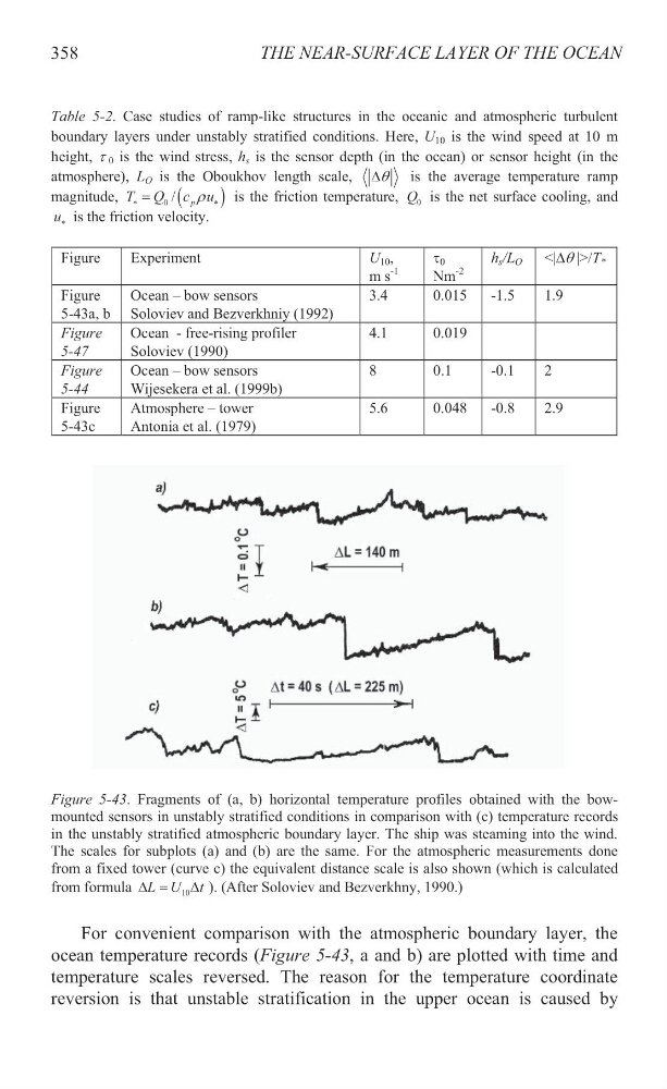
Figure 5-43. Fragments of (a, b) horizontal temperature profiles obtained with the bowmounted sensors in unstably stratified conditions in comparison with (c) temperature records
in the unstably stratified atmospheric boundary layer. The ship was steaming into the wind.
The scales for subplots (a) and (b) are the same. For the atmospheric measurements done
from a fixed tower (curve c) the equivalent distance scale is also shown (which is calculated
from formula
10
L U t
'
' ). (After Soloviev and Bezverkhny, 1990.)
For convenient comparison with the atmospheric boundary layer, the
ocean temperature records (Figure 5-43, a and b) are plotted with time and
temperature scales reversed. The reason for the temperature coordinate
reversion is that unstable stratification in the upper ocean is caused by
358
Table 5-2. Case studies of ramp-like structures in the oceanic and atmospheric turbulent
boundary layers under unstably stratified conditions. Here, U 10 is the wind speed at 10 m
height, W 0 is the wind stress, h s is the sensor depth (in the ocean) or sensor height (in the
atmosphere), L O is the Oboukhov length scale,
T
'
is the average temperature ramp
magnitude,
0 / p
T Q c u
U
is the friction temperature, 0
Q is the net surface cooling, and
u is the friction velocity.
Figure
Experiment
U 10 ,
m s
-1
W
Nm
-2
h s /L O <|'T_>/T *
Figure
5-43a, b
Ocean – bow sensors
Soloviev and Bezverkhniy (1992)
3.4
0.015
-1.5
1.9
Figure
5-47
Ocean - free-rising profiler
Soloviev (1990)
4.1
0.019
Figure
5-44
Ocean – bow sensors
Wijesekera et al. (1999b)
8
0.1
-0.1
2
Figure
5-43c
Atmosphere – tower
Antonia et al. (1979)
5.6
0.048
-0.8
2.9
Figure 5-43. Fragments of (a, b) horizontal temperature profiles obtained with the bowmounted sensors in unstably stratified conditions in comparison with (c) temperature records
in the unstably stratified atmospheric boundary layer. The ship was steaming into the wind.
The scales for subplots (a) and (b) are the same. For the atmospheric measurements done
from a fixed tower (curve c) the equivalent distance scale is also shown (which is calculated
from formula
10
L U t
'
' ). (After Soloviev and Bezverkhny, 1990.)
For convenient comparison with the atmospheric boundary layer, the
ocean temperature records (Figure 5-43, a and b) are plotted with time and
temperature scales reversed. The reason for the temperature coordinate
reversion is that unstable stratification in the upper ocean is caused by
358