

364 Nadia Pinardi et al.
large-scale models make use of no-slip boundary conditions, e.g. Îl ::; O, along the
domain rigid walls and/or have a series of sponge layers where temperature and
salinity are fixed to climatological values. These sponge layers may parameterize
unresolved physics (such as water-ice interactions at high latitudes), parts of
oceans connected through narrow straits to the large-scale basin of interest and
parts of ocean basins dynamically uncoupled on the time scales of interest. This is
the case for example of the Atlantic ocean and the Mediterranean Sea, connected
by the narrow Gibraltar Strait, the Atlantic with the Gulf of Mexico Strait, the
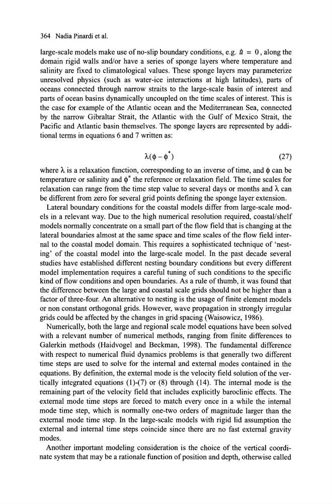
Pacific and Atlantic basin themselves. The sponge layers are represented by additional terms in equations 6 and 7 written as:
•
A( <1> - <1> )
(27)
where A is a relaxation function, corresponding to an inverse of time, and <1> can be
temperature or salinity and <1>* the reference or relaxation field. The time scales for
relaxation can range from the time step value to several days or months and A can
be different from zero for several grid points defining the sponge layer extension.
Lateral boundary conditions for the coastal models differ from large-scale models in a relevant way. Due to the high numerical resolution required, coastal/shelf
models normally concentrate on a small part of the flow field that is changing at the
lateral boundaries almost at the same space and time scales ofthe flow field internal to the coastal model domain. This requires a sophisticated technique of 'nesting' of the coastal model into the large-scale model. In the past decade several
studies have established different nesting boundary conditions but every different
model implementation requires a careful tuning of such conditions to the specific
kind of flow conditions and open boundaries. As a rule of thumb, it was found that
the difference between the large and coastal scale grids should not be higher than a
factor of three-four. An alternative to nesting is the usage of finite element models
or non constant orthogonal grids. However, wave propagation in strongly irregular
grids could be affected by the changes in grid spacing (Waisowicz, 1986).
Numerically, both the large and regional scale model equations have been solved
with a relevant number of numeric al methods, ranging from finite differences to
Galerkin methods (Haidvogel and Beckman, 1998). The fundamental difference
with respect to numerical fluid dynamics problems is that generally two different
time steps are used to solve for the internal and external modes contained in the
equations. By definition, the external mode is the velocity field solution ofthe vertically integrated equations (1)-(7) or (8) through (14). The internal mode is the
remaining part of the velocity field that includes explicitly baroclinic effects. The
external mode time steps are forced to match every once in a while the internal
mode time step, which is normally one-two orders of magnitude larger than the
external mode time step. In the large-scale models with rigid lid assumption the
external and internal time steps coincide since there are no fast external gravity
modes.
Another important modeling consideration is the choice of the vertical coordinate system that may be a rationale function of position and depth, otherwise called
large-scale models make use of no-slip boundary conditions, e.g. Îl ::; O, along the
domain rigid walls and/or have a series of sponge layers where temperature and
salinity are fixed to climatological values. These sponge layers may parameterize
unresolved physics (such as water-ice interactions at high latitudes), parts of
oceans connected through narrow straits to the large-scale basin of interest and
parts of ocean basins dynamically uncoupled on the time scales of interest. This is
the case for example of the Atlantic ocean and the Mediterranean Sea, connected
by the narrow Gibraltar Strait, the Atlantic with the Gulf of Mexico Strait, the
Pacific and Atlantic basin themselves. The sponge layers are represented by additional terms in equations 6 and 7 written as:
•
A( <1> - <1> )
(27)
where A is a relaxation function, corresponding to an inverse of time, and <1> can be
temperature or salinity and <1>* the reference or relaxation field. The time scales for
relaxation can range from the time step value to several days or months and A can
be different from zero for several grid points defining the sponge layer extension.
Lateral boundary conditions for the coastal models differ from large-scale models in a relevant way. Due to the high numerical resolution required, coastal/shelf
models normally concentrate on a small part of the flow field that is changing at the
lateral boundaries almost at the same space and time scales ofthe flow field internal to the coastal model domain. This requires a sophisticated technique of 'nesting' of the coastal model into the large-scale model. In the past decade several
studies have established different nesting boundary conditions but every different
model implementation requires a careful tuning of such conditions to the specific
kind of flow conditions and open boundaries. As a rule of thumb, it was found that
the difference between the large and coastal scale grids should not be higher than a
factor of three-four. An alternative to nesting is the usage of finite element models
or non constant orthogonal grids. However, wave propagation in strongly irregular
grids could be affected by the changes in grid spacing (Waisowicz, 1986).
Numerically, both the large and regional scale model equations have been solved
with a relevant number of numeric al methods, ranging from finite differences to
Galerkin methods (Haidvogel and Beckman, 1998). The fundamental difference
with respect to numerical fluid dynamics problems is that generally two different
time steps are used to solve for the internal and external modes contained in the
equations. By definition, the external mode is the velocity field solution ofthe vertically integrated equations (1)-(7) or (8) through (14). The internal mode is the
remaining part of the velocity field that includes explicitly baroclinic effects. The
external mode time steps are forced to match every once in a while the internal
mode time step, which is normally one-two orders of magnitude larger than the
external mode time step. In the large-scale models with rigid lid assumption the
external and internal time steps coincide since there are no fast external gravity
modes.
Another important modeling consideration is the choice of the vertical coordinate system that may be a rationale function of position and depth, otherwise called