

Toward Marine Environmental Predictions in the Mediterranean Sea Coastal Areas
365
a bottom following coordinate system. The most commonly used transformed
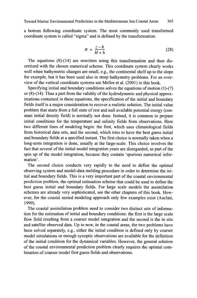
coordinate system is called "sigma" and is defined by the transformation:
z-h
cr = - -
H+h
(28)
The equations (8)-(14) are rewritten using this transformation and then discretized with the chosen numerical scheme. This coordinate system c1early works
well when bathymetric changes are small, e.g., the continental shelfup to the slope
for example, but it has been used also in steep bathymetry problems. For an overview of the vertical coordinate systems see Mellor et al. (2001) in this book.
Specifying initial and boundary conditions solves the equations of motion (1 )-(7)
or (8)-(14). Thus a part from the validity ofthe hydrodynamic and physical approximations contained in these equations, the specification of the initial and boundary
fields itself is a major consideration to recover a realistic solution. The initial value
problem that starts from a fuU state of rest and nuU available potential energy (constant initial density field) is normally not done. Instead, it is common to prepare
initial conditions for the temperature and salinity fields from observations. Here
two different lines of modeling begin: the first, which uses climatological fields
from historical data sets, and the second, which tries to have the best guess initial
and boundary fields at a specified instant. The first choice is normaUy taken when a
long-term integration is done, usuaUy at the large-scale. This choice involves the
fact that several of the initial model integration years are disregarded, as part of the
spin up of the model integration, because they contain 'spurious numeric al information'.
The second choice conducts very rapidly to the need to de fine the optimal
observing system and model-data melding procedure in order to determine the initial and boundary fields. This is a very important part of the coastal environmental
prediction problem, the optimal estimation scheme that could be used to define the
best guess initial and boundary fields. For large scale models the assimilation
schemes are already very sophisticated, see the other chapters of this book. However, for the coastal nested modeling approach only few examples exist (Auclair,
1999).
The coastal assimilation problem need to consider two distinct sets of information for the estimation of initial and boundary conditions: the first is the large scale
flow field resulting from a coarser model integration and the second is the in situ
and satellite observed data. Up to now, in the coastal areas, the two problems have
been solved separately, e.g., either the initial condition is defined only by coarser
model simulations or enough synoptic observations are available for the definition
of the initial condition for the dynamical variables. However, the general solution
of the coastal environmental prediction problem clearly requires the optimal combination of coarser model first guess fields and observations.
365
a bottom following coordinate system. The most commonly used transformed
coordinate system is called "sigma" and is defined by the transformation:
z-h
cr = - -
H+h
(28)
The equations (8)-(14) are rewritten using this transformation and then discretized with the chosen numerical scheme. This coordinate system c1early works
well when bathymetric changes are small, e.g., the continental shelfup to the slope
for example, but it has been used also in steep bathymetry problems. For an overview of the vertical coordinate systems see Mellor et al. (2001) in this book.
Specifying initial and boundary conditions solves the equations of motion (1 )-(7)
or (8)-(14). Thus a part from the validity ofthe hydrodynamic and physical approximations contained in these equations, the specification of the initial and boundary
fields itself is a major consideration to recover a realistic solution. The initial value
problem that starts from a fuU state of rest and nuU available potential energy (constant initial density field) is normally not done. Instead, it is common to prepare
initial conditions for the temperature and salinity fields from observations. Here
two different lines of modeling begin: the first, which uses climatological fields
from historical data sets, and the second, which tries to have the best guess initial
and boundary fields at a specified instant. The first choice is normaUy taken when a
long-term integration is done, usuaUy at the large-scale. This choice involves the
fact that several of the initial model integration years are disregarded, as part of the
spin up of the model integration, because they contain 'spurious numeric al information'.
The second choice conducts very rapidly to the need to de fine the optimal
observing system and model-data melding procedure in order to determine the initial and boundary fields. This is a very important part of the coastal environmental
prediction problem, the optimal estimation scheme that could be used to define the
best guess initial and boundary fields. For large scale models the assimilation
schemes are already very sophisticated, see the other chapters of this book. However, for the coastal nested modeling approach only few examples exist (Auclair,
1999).
The coastal assimilation problem need to consider two distinct sets of information for the estimation of initial and boundary conditions: the first is the large scale
flow field resulting from a coarser model integration and the second is the in situ
and satellite observed data. Up to now, in the coastal areas, the two problems have
been solved separately, e.g., either the initial condition is defined only by coarser
model simulations or enough synoptic observations are available for the definition
of the initial condition for the dynamical variables. However, the general solution
of the coastal environmental prediction problem clearly requires the optimal combination of coarser model first guess fields and observations.