

288 Pierre De Mey and Mounir Benkiran
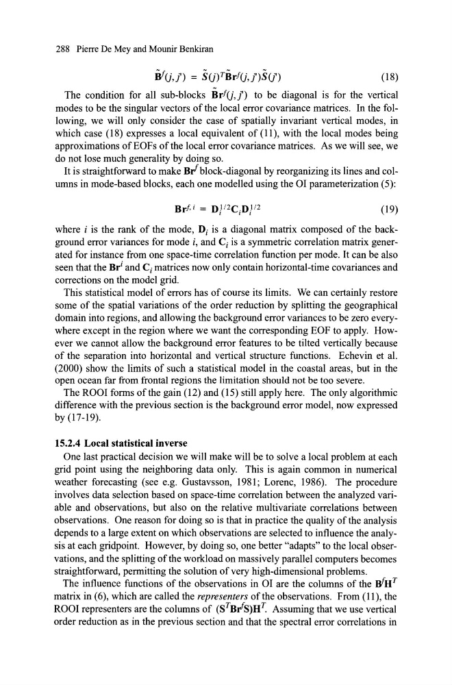
(18)
The condition for aH sub-blocks BrfU, j') to be diagonal is for the vertical
modes to be the singular vectors ofthe local error covariance matrices. In the following, we will only consider the case of spatiaHy invariant vertical modes, in
which case (18) expresses a local equivalent of (11), with the local modes being
approximations ofEOFs ofthe local error covariance matrices. As we will see, we
do not Iose much generality by doing so.
It is straightforward to make BI block-diagonal by reorganizing its lines and columns in mode-based blocks, each one modelled using the OI parameterization (5):
(19)
where i is the rank of the mode, Di is a diagonal matrix composed of the background error variances for mode i, and Ci is a symmetric correlation matrix generated for instance from one space-time correlation function per mode. It can be also
seen that the Br i and Ci matrices now only contain horizontal-time covariances and
corrections on the model grid.
This statistical model of errors has of course its limits. We can certainly restore
some of the spatial variations of the order reduction by splitting the geographical
domain into regions, and allowing the background error variances to be zero everywhere except in the region where we want the corresponding EOF to apply. However we cannot allow the background error features to be tilted vertically because
of the separation into horizontal and vertical structure functions. Echevin et al.
(2000) show the limits of such a statistic al model in the coastal areas, but in the
open ocean far from frontal regions the limitation should not be too severe.
The ROOI forms ofthe gain (12) and (15) stiH apply here. The only algorithmic
difference with the previous section is the background error model, now expressed
by (17-19).
15.2.4 Local statistical inverse
One last practical decision we will make will be to solve a local problem at each
grid point using the neighboring data only. This is again common in numerical
weather forecasting (see e.g. Gustavsson, 1981; Lorenc, 1986). The procedure
involves data selection based on space-time correlation between the analyzed variable and observations, but also on the relative multivariate correlations between
observations. One reason for doing so is that in practice the quality of the analysis
depends to a large extent on which observations are selected to influence the analysis at each gridpoint. However, by do ing so, one better "adapts" to the local observations, and the splitting ofthe workload on massively parallel computers becomes
straightforward, permitting the solution ofvery high-dimensional problems.
The influence functions of the observations in OI are the columns of the WH T
matrix in (6), which are called the representers ofthe observations. From (11), the
ROOI representers are the columns of (STBIS)H~ Assuming that we use vertical
order reduction as in the previous section and that the spectral error correlations in
(18)
The condition for aH sub-blocks BrfU, j') to be diagonal is for the vertical
modes to be the singular vectors ofthe local error covariance matrices. In the following, we will only consider the case of spatiaHy invariant vertical modes, in
which case (18) expresses a local equivalent of (11), with the local modes being
approximations ofEOFs ofthe local error covariance matrices. As we will see, we
do not Iose much generality by doing so.
It is straightforward to make BI block-diagonal by reorganizing its lines and columns in mode-based blocks, each one modelled using the OI parameterization (5):
(19)
where i is the rank of the mode, Di is a diagonal matrix composed of the background error variances for mode i, and Ci is a symmetric correlation matrix generated for instance from one space-time correlation function per mode. It can be also
seen that the Br i and Ci matrices now only contain horizontal-time covariances and
corrections on the model grid.
This statistical model of errors has of course its limits. We can certainly restore
some of the spatial variations of the order reduction by splitting the geographical
domain into regions, and allowing the background error variances to be zero everywhere except in the region where we want the corresponding EOF to apply. However we cannot allow the background error features to be tilted vertically because
of the separation into horizontal and vertical structure functions. Echevin et al.
(2000) show the limits of such a statistic al model in the coastal areas, but in the
open ocean far from frontal regions the limitation should not be too severe.
The ROOI forms ofthe gain (12) and (15) stiH apply here. The only algorithmic
difference with the previous section is the background error model, now expressed
by (17-19).
15.2.4 Local statistical inverse
One last practical decision we will make will be to solve a local problem at each
grid point using the neighboring data only. This is again common in numerical
weather forecasting (see e.g. Gustavsson, 1981; Lorenc, 1986). The procedure
involves data selection based on space-time correlation between the analyzed variable and observations, but also on the relative multivariate correlations between
observations. One reason for doing so is that in practice the quality of the analysis
depends to a large extent on which observations are selected to influence the analysis at each gridpoint. However, by do ing so, one better "adapts" to the local observations, and the splitting ofthe workload on massively parallel computers becomes
straightforward, permitting the solution ofvery high-dimensional problems.
The influence functions of the observations in OI are the columns of the WH T
matrix in (6), which are called the representers ofthe observations. From (11), the
ROOI representers are the columns of (STBIS)H~ Assuming that we use vertical
order reduction as in the previous section and that the spectral error correlations in