

A Multivariate Reduced-order Optimal Interpolation Method and its Application
289
Ci vanish after some distance, it is clear that the ROOI representers can only be
made local if the observation operators are local. In practice, there are three kinds
of observation operators in the ocean: vertical observation operators (e.g. temperature, salinity, density profiles), operators based on local gradients (e.g. geostrophic
velocities), and global observation operators (e.g. surface pressure and sea-level
anomaly in most rigid-lid models). Therefore if we wish to solve local inverse
problems we have to exclude the last category. However, the sea-level anomaly
(SLA) observation operator can be considered to be local in some cases such as the
following:
(1) If the model is a rigid-lid model, if only the geostrophic contribution to SLA
is subject to errors in the model, and if errors can be considered small below some
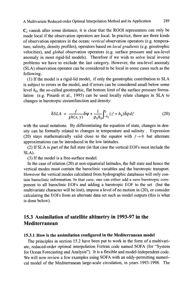
level ha, the so-called geostrophic, flat bottom limit of the surface pressure formulation (e.g. Pinardi et al., 1995) can be used locally relate changes in SLA to
changes in barotropic streamfunction and density:
oSLA = f O\jf + -l-fo (z' + ho)opdz'
gh(x, y)
POh O -ha
(20)
with the usual notations. By differentiating the equation of state, changes in density can be formally related to changes in temperature and salinity. Expression
(20) stays mathematically valid close to the equator with f --t O but alternate
approximations can be introduced in the low latitudes.
(2) IfSLA is part ofthe full state (in that case the vertical EOFs must include the
SLA).
(3) Ifthe model is a free-surface model.
In the case ofrelation (20) at non-equatoriallatitudes, the full state and hence the
vertical modes must contain the baroclinic variables and the barotropic transport.
However the vertical modes calculated from hydrographic databases will only contain baroclinic information. In that case, one can either add a zero barotropic component to all baroclinic EOFs and adding a barotropic EOF to the set (but the
multi variate character will be lost), impose a level of no motion in (20), or consider
calculating the EOFs from an alternate data set such as model outputs (this is what
is done below).
15.3 Assimilation of satellite altimetry in 1993-97 in the
Mediterranean
15.3.1 How is the assimilation configured in the Mediterranean model
The principles in section 15.2 have been put to work in the form of a multivariate, reduced-order optimal interpolation Fortran code named SOFA (for "System
for Ocean Forecasting and Analysis"). It is a flexible and model-independent code.
We will now review a few examples using SOFA with an eddy-permitting numerical model of the Mediterranean large-scale circulation, in years 1993-1998. The
289
Ci vanish after some distance, it is clear that the ROOI representers can only be
made local if the observation operators are local. In practice, there are three kinds
of observation operators in the ocean: vertical observation operators (e.g. temperature, salinity, density profiles), operators based on local gradients (e.g. geostrophic
velocities), and global observation operators (e.g. surface pressure and sea-level
anomaly in most rigid-lid models). Therefore if we wish to solve local inverse
problems we have to exclude the last category. However, the sea-level anomaly
(SLA) observation operator can be considered to be local in some cases such as the
following:
(1) If the model is a rigid-lid model, if only the geostrophic contribution to SLA
is subject to errors in the model, and if errors can be considered small below some
level ha, the so-called geostrophic, flat bottom limit of the surface pressure formulation (e.g. Pinardi et al., 1995) can be used locally relate changes in SLA to
changes in barotropic streamfunction and density:
oSLA = f O\jf + -l-fo (z' + ho)opdz'
gh(x, y)
POh O -ha
(20)
with the usual notations. By differentiating the equation of state, changes in density can be formally related to changes in temperature and salinity. Expression
(20) stays mathematically valid close to the equator with f --t O but alternate
approximations can be introduced in the low latitudes.
(2) IfSLA is part ofthe full state (in that case the vertical EOFs must include the
SLA).
(3) Ifthe model is a free-surface model.
In the case ofrelation (20) at non-equatoriallatitudes, the full state and hence the
vertical modes must contain the baroclinic variables and the barotropic transport.
However the vertical modes calculated from hydrographic databases will only contain baroclinic information. In that case, one can either add a zero barotropic component to all baroclinic EOFs and adding a barotropic EOF to the set (but the
multi variate character will be lost), impose a level of no motion in (20), or consider
calculating the EOFs from an alternate data set such as model outputs (this is what
is done below).
15.3 Assimilation of satellite altimetry in 1993-97 in the
Mediterranean
15.3.1 How is the assimilation configured in the Mediterranean model
The principles in section 15.2 have been put to work in the form of a multivariate, reduced-order optimal interpolation Fortran code named SOFA (for "System
for Ocean Forecasting and Analysis"). It is a flexible and model-independent code.
We will now review a few examples using SOFA with an eddy-permitting numerical model of the Mediterranean large-scale circulation, in years 1993-1998. The