

158 Mojib Latif, Axei Timmermann, Anselm Grotzner, Christian Eckert, Reinhard Voss
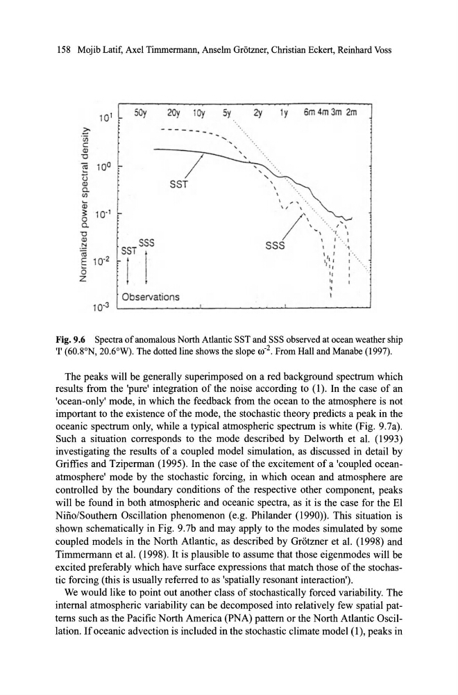
Fig.9.6 Spectra of anomalous North Atlantic SST and SSS observed at ocean weather ship
'1' (60.8°N, 20.6°W). The dotted line shows the slope 0)-2. From HalI and Manabe (1997).
The peaks will be generally superimposed on a red background spectrum which
results from the 'pure' integration of the noise according to (1). In the case of an
'ocean-on1y' mode, in which the feedback from the ocean to the atmosphere is not
important to the existence of the mode, the stochastic theory predicts a peak in the
oceanic spectrum on1y, whi1e a typica1 atmospheric spectrum is white (Fig. 9.7a).
Such a situation corresponds to the mode described by De1worth et al. (1993)
investigating the results of a coupled model simulation, as discussed in detail by
Griffies and Tziperman (1995). In the case of the excitement of a 'coup1ed oceanatmosphere' mode by the stochastic forcing, in which ocean and atmosphere are
controlled by the boundary conditions of the respective other component, peaks
will be found in both atmospheric and oceanic spectra, as it is the case for the El
Nifio/Southern Oscillation phenomenon (e.g. Philander (1990)). This situation is
shown schematically in Fig. 9.7b and may apply to the modes simulated by some
coupled models in the North Atlantic, as described by Gr6tzner et al. (1998) and
Timmermann et al. (1998). It is plausible to assume that those eigenmodes will be
excited preferably which have surface expressions that match those of the stochastic forcing (this is usually referred to as 'spatially resonant interaction').
We would like to point out another c\ass of stochastically forced variability. The
internal atmospheric variability can be decomposed into relatively few spatial patterns such as the Pacific North America (PNA) pattern or the North Atlantic Oscillation. If oceanic advection is inc\uded in the stochastic c\imate model (1), peaks in
Fig.9.6 Spectra of anomalous North Atlantic SST and SSS observed at ocean weather ship
'1' (60.8°N, 20.6°W). The dotted line shows the slope 0)-2. From HalI and Manabe (1997).
The peaks will be generally superimposed on a red background spectrum which
results from the 'pure' integration of the noise according to (1). In the case of an
'ocean-on1y' mode, in which the feedback from the ocean to the atmosphere is not
important to the existence of the mode, the stochastic theory predicts a peak in the
oceanic spectrum on1y, whi1e a typica1 atmospheric spectrum is white (Fig. 9.7a).
Such a situation corresponds to the mode described by De1worth et al. (1993)
investigating the results of a coupled model simulation, as discussed in detail by
Griffies and Tziperman (1995). In the case of the excitement of a 'coup1ed oceanatmosphere' mode by the stochastic forcing, in which ocean and atmosphere are
controlled by the boundary conditions of the respective other component, peaks
will be found in both atmospheric and oceanic spectra, as it is the case for the El
Nifio/Southern Oscillation phenomenon (e.g. Philander (1990)). This situation is
shown schematically in Fig. 9.7b and may apply to the modes simulated by some
coupled models in the North Atlantic, as described by Gr6tzner et al. (1998) and
Timmermann et al. (1998). It is plausible to assume that those eigenmodes will be
excited preferably which have surface expressions that match those of the stochastic forcing (this is usually referred to as 'spatially resonant interaction').
We would like to point out another c\ass of stochastically forced variability. The
internal atmospheric variability can be decomposed into relatively few spatial patterns such as the Pacific North America (PNA) pattern or the North Atlantic Oscillation. If oceanic advection is inc\uded in the stochastic c\imate model (1), peaks in