

Sequential Data Assimilation for Nonlinear Dynamics: The Ensemble Kalman Filter
107
[
(Xl -X 2 )2
J
P(X I - X2) = exp
z2
.
(28)
This distribution will be called ('l') where the functions 'l' have been discretized on the numerical grid.
2
o
- 1
-2
o
5
10
15
20
0.8
0.6
0.4
25
30
x-coordinate
x-coordinate
KF analysis -
EnKF anaJysis 100
EnKF anaJysis 500 ----.. .
EnKF analysis 1000 ....... .
35
40
45
KF variance. K F -
En KF variance. 100
EnK.F variance, 500 ...... -
EnKF variance. 1000 ...... ..
50
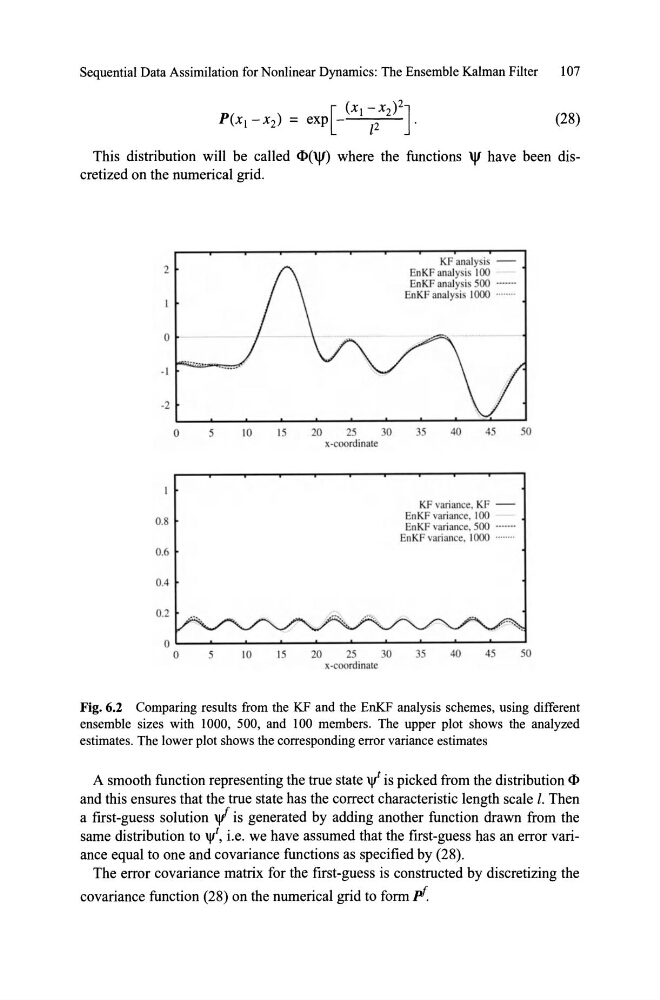
Fig. 6.2 Comparing results from the KF and the EnKF analysis schemes, using different
ensemble sizes with 1000, 500, and 100 members. The upper plot shows the analyzed
estimates. The lower plot shows the corresponding error variance estimates
A smooth function representing the true state 'V! is picked from the distribution <1>
and this ensures that the true state has the correct characteristic length scale 1. Then
a first-guess solution '" is generated by adding another function drawn from the
same distribution to ~, i.e. we have assumed that the first-guess has an error variance equal to one and covariance functions as specified by (28).
The error covariance matrix for the first-guess is constructed by discretizing the
covariance function (28) on the numerical grid to form P.
107
[
(Xl -X 2 )2
J
P(X I - X2) = exp
z2
.
(28)
This distribution will be called ('l') where the functions 'l' have been discretized on the numerical grid.
2
o
- 1
-2
o
5
10
15
20
0.8
0.6
0.4
25
30
x-coordinate
x-coordinate
KF analysis -
EnKF anaJysis 100
EnKF anaJysis 500 ----.. .
EnKF analysis 1000 ....... .
35
40
45
KF variance. K F -
En KF variance. 100
EnK.F variance, 500 ...... -
EnKF variance. 1000 ...... ..
50
Fig. 6.2 Comparing results from the KF and the EnKF analysis schemes, using different
ensemble sizes with 1000, 500, and 100 members. The upper plot shows the analyzed
estimates. The lower plot shows the corresponding error variance estimates
A smooth function representing the true state 'V! is picked from the distribution <1>
and this ensures that the true state has the correct characteristic length scale 1. Then
a first-guess solution '" is generated by adding another function drawn from the
same distribution to ~, i.e. we have assumed that the first-guess has an error variance equal to one and covariance functions as specified by (28).
The error covariance matrix for the first-guess is constructed by discretizing the
covariance function (28) on the numerical grid to form P.