

108 Geir Evensen
There are 10 measurements distributed at regular intervals in x. Each measurement is generated by measuring the true state ~ and then adding Gaussian distributed noise with mean zero and variance 0.2.
An ensemble representing the error variance equal to one is now generated by
adding functions drawn from <1> to the first-guess. Here 1000 members were used in
the ensemble. Thus, we now have a first-guess estimate of the true state with the
error covariance represented by the ensemble.
The results from this example are given in Fig. 6.1. The ensemble estimates are
of course the means of the analyzed ensembles. By comparing the KF and the
EnKF estimates it is clear that EnKF gives a consistent analysis \f. The lower plot
shows the corresponding error variances. The upper line is the initial error variance
for the first-guess equal to one. Then there are two error variance estimates corresponding to the EnKF and the standard Kalman filter. Clearly, the EnKF analysis
scheme provides an error variance estimate which is very close to the one which
follows from the standard Kalman filter.
In Fig. 6.1 we examine the sensitivity of the analysis scheme with respect to the
size ofthe ensemble. Clearly there is not a big difference in the estimates using 100
or 1000 ensemble members.
6.5 A highly nonlinear case: the Lorenz equations
An example is now given using the highly nonlinear and chaotic Lorenz equations. The celebrated Lorenz model has been subject of extensive studies motivated
by its chaotic and strongly nonlinear nature. In the field of data assimilation, the
model has served as a testbed for examining the properties ofvarious data assimilation methods when used with strongly nonlinear dynamics. The results have been
used to suggest properties and possibilities of the methods for applications with
oceanic and atmospheric models which may also be strongly nonlinear and chaotic.
6.5.1 Model Equations
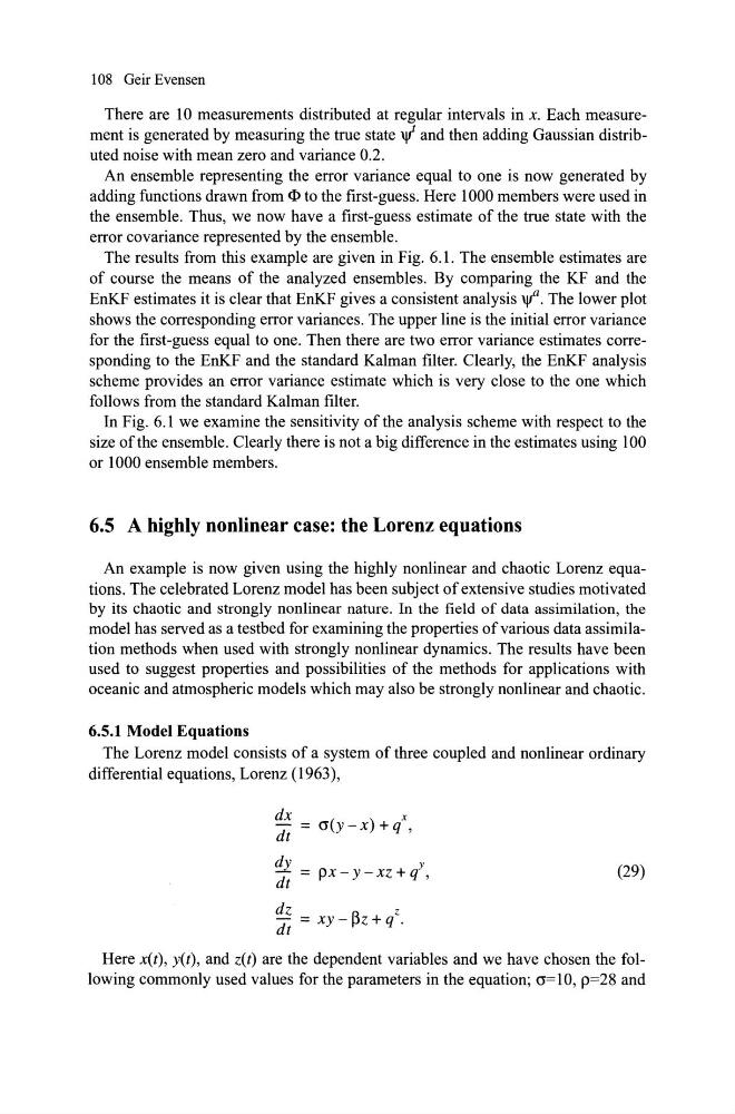
The Lorenz model consists of a system of three coupled and nonlinear ordinary
differential equations, Lorenz (1963),
dx
x
dt = a(y - x) + q ,
d: = px - y - xz + l,
dz
R
Z
dt = xy - pZ + q .
(29)
Here x(t), y(t), and z(t) are the dependent variables and we have chosen the following commonly used values for the parameters in the equation; a=10, p=28 and
There are 10 measurements distributed at regular intervals in x. Each measurement is generated by measuring the true state ~ and then adding Gaussian distributed noise with mean zero and variance 0.2.
An ensemble representing the error variance equal to one is now generated by
adding functions drawn from <1> to the first-guess. Here 1000 members were used in
the ensemble. Thus, we now have a first-guess estimate of the true state with the
error covariance represented by the ensemble.
The results from this example are given in Fig. 6.1. The ensemble estimates are
of course the means of the analyzed ensembles. By comparing the KF and the
EnKF estimates it is clear that EnKF gives a consistent analysis \f. The lower plot
shows the corresponding error variances. The upper line is the initial error variance
for the first-guess equal to one. Then there are two error variance estimates corresponding to the EnKF and the standard Kalman filter. Clearly, the EnKF analysis
scheme provides an error variance estimate which is very close to the one which
follows from the standard Kalman filter.
In Fig. 6.1 we examine the sensitivity of the analysis scheme with respect to the
size ofthe ensemble. Clearly there is not a big difference in the estimates using 100
or 1000 ensemble members.
6.5 A highly nonlinear case: the Lorenz equations
An example is now given using the highly nonlinear and chaotic Lorenz equations. The celebrated Lorenz model has been subject of extensive studies motivated
by its chaotic and strongly nonlinear nature. In the field of data assimilation, the
model has served as a testbed for examining the properties ofvarious data assimilation methods when used with strongly nonlinear dynamics. The results have been
used to suggest properties and possibilities of the methods for applications with
oceanic and atmospheric models which may also be strongly nonlinear and chaotic.
6.5.1 Model Equations
The Lorenz model consists of a system of three coupled and nonlinear ordinary
differential equations, Lorenz (1963),
dx
x
dt = a(y - x) + q ,
d: = px - y - xz + l,
dz
R
Z
dt = xy - pZ + q .
(29)
Here x(t), y(t), and z(t) are the dependent variables and we have chosen the following commonly used values for the parameters in the equation; a=10, p=28 and