

106 Geir Evensen
6.4 An example of the analysis scheme
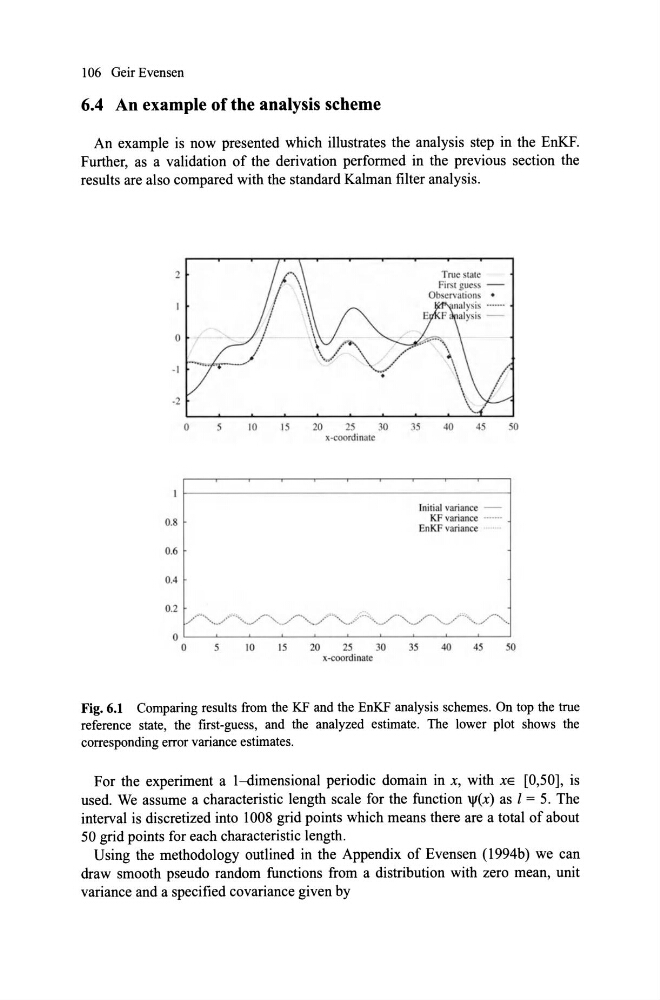
An example is now presented which iIIustrates the analysis step in the EnKF.
Further, as a validation of the derivation performed in the previous section the
results are also compared with the standard Kalman filter analysis.
2
o
· 1
-2
0.8
0.6
0.4
0.2
o
5
10
15
20
25
x-coordin alC
30
35
40
45
50
Initial variance -
KF variance ..... _.
EnKF variance "".
V~"··'· .. ../··"';·;'r •• ""/'-·'./~ .• ,-", •• ";J""',-.. $-';'::"'.~,-",/·"""" . .,.../, .. _"'-.,.......-';: ... ;Ot,. . ............ ...-. , ••
10
15
20
25
30
35
40
45
50
x-coordinale
Fig. 6_1 Comparing results from the KF and the EnKF analysis schemes. On top the true
reference state, the first-guess, and the analyzed estimate. The lower plot shows the
corresponding error variance estimates.
For the experiment a l-dimensional periodic domain in x, with XE [0,50], is
used. We assume a characteristic length scale for the function \jI(x) as 1 = 5. The
interval is discretized into 1008 grid points which means there are a total of about
50 grid points for each characteristic length.
Using the methodology outlined in the Appendix of Evensen (1994b) we can
draw smooth pseudo random functions from a distribution with zero mean, unit
variance and a specified covariance given by
6.4 An example of the analysis scheme
An example is now presented which iIIustrates the analysis step in the EnKF.
Further, as a validation of the derivation performed in the previous section the
results are also compared with the standard Kalman filter analysis.
2
o
· 1
-2
0.8
0.6
0.4
0.2
o
5
10
15
20
25
x-coordin alC
30
35
40
45
50
Initial variance -
KF variance ..... _.
EnKF variance "".
V~"··'· .. ../··"';·;'r •• ""/'-·'./~ .• ,-", •• ";J""',-.. $-';'::"'.~,-",/·"""" . .,.../, .. _"'-.,.......-';: ... ;Ot,. . ............ ...-. , ••
10
15
20
25
30
35
40
45
50
x-coordinale
Fig. 6_1 Comparing results from the KF and the EnKF analysis schemes. On top the true
reference state, the first-guess, and the analyzed estimate. The lower plot shows the
corresponding error variance estimates.
For the experiment a l-dimensional periodic domain in x, with XE [0,50], is
used. We assume a characteristic length scale for the function \jI(x) as 1 = 5. The
interval is discretized into 1008 grid points which means there are a total of about
50 grid points for each characteristic length.
Using the methodology outlined in the Appendix of Evensen (1994b) we can
draw smooth pseudo random functions from a distribution with zero mean, unit
variance and a specified covariance given by