

Sequential Data Assimilation for Nonlinear Dynamics: The Ensemble Kalman Filter
103
Another alternative approach for solving the Fokker-Planck equation and predicting the error statistics is to use Monte-Carlo methods. If a probability density
function is represented by a large ensemble of model states, it is possible to integrate each member forward in time using the stochastic model (17). Thus, integrating an ensemble of model states becomes equivalent to solving the Fokker-Planck
equation using aMonte Carlo method.
The standard approach is to first calculate a best guess initial condition based on
information available from data and statistics. An ensemble of initial states is then
generated in which the mean equals the best guess initial condition and the variance is specified on the basis ofknowledge ofthe uncertainty in the first-guess initial state. The covariance or smoothness of the ensemble should reflect the true
scales of the system.
The effect of external error growth must be included to give reliable estimates for
the evolution of errors. In the Kalman filter this can be done rather simply by adding the system error covariance matrix every time step. However, in the MonteCarlo method, each ensemble member is integrated as a stochastic differential
equation and is forced by smooth pseudo-random fields with a specified variance
and covariance to simulate the model errors. This will provide a realistic increase
in the ensemble variance provided that the estimate of the model error variance is
reasonably good.
6.3.3 An analysis scheme
The Kalman Filter (KF) analysis scheme was based on the definitions of pf and
pa as given by equations (12) and (13). We will now give a new derivation ofthe
analysis scheme where the ensemble covariances are used as defined by (14) and
(15). This is convenient since in practical implementations one is doing exactly
this, and it will also lead to a consistent formulation of the EnKF.
As will be shown later it is essential that the observations are treated as random
variables having a distribution with mean equal to the first-guess observations and
covariance equal to R . Thus, we start by defining an ensemble of observations
(19)
where j counts from 1 to the number of model state ensemble members. Next we
define the ensemble covariance matrix of the measurements as
-T
Re = ee ,
(20)
and of course in the limit of an infinite ensemble, this matrix will converge towards
the prescribed error covariance matrix R used in the standard Kalman filter.
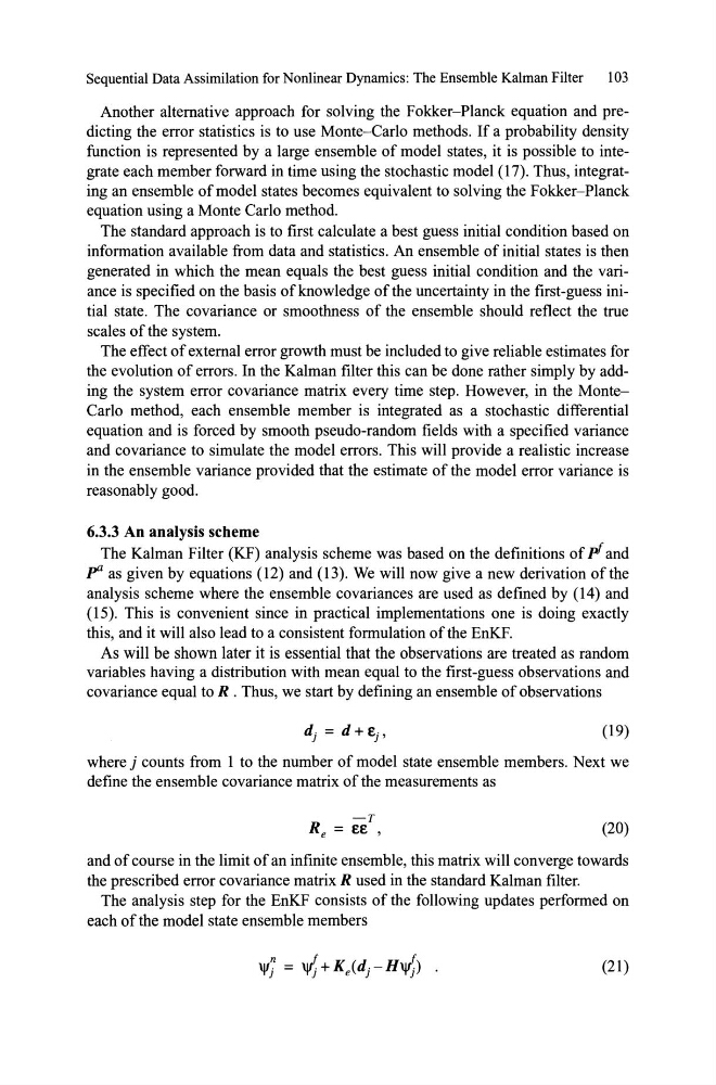
The analysis step for the EnKF consists of the following updates performed on
each ofthe model state ensemble members
(21)
103
Another alternative approach for solving the Fokker-Planck equation and predicting the error statistics is to use Monte-Carlo methods. If a probability density
function is represented by a large ensemble of model states, it is possible to integrate each member forward in time using the stochastic model (17). Thus, integrating an ensemble of model states becomes equivalent to solving the Fokker-Planck
equation using aMonte Carlo method.
The standard approach is to first calculate a best guess initial condition based on
information available from data and statistics. An ensemble of initial states is then
generated in which the mean equals the best guess initial condition and the variance is specified on the basis ofknowledge ofthe uncertainty in the first-guess initial state. The covariance or smoothness of the ensemble should reflect the true
scales of the system.
The effect of external error growth must be included to give reliable estimates for
the evolution of errors. In the Kalman filter this can be done rather simply by adding the system error covariance matrix every time step. However, in the MonteCarlo method, each ensemble member is integrated as a stochastic differential
equation and is forced by smooth pseudo-random fields with a specified variance
and covariance to simulate the model errors. This will provide a realistic increase
in the ensemble variance provided that the estimate of the model error variance is
reasonably good.
6.3.3 An analysis scheme
The Kalman Filter (KF) analysis scheme was based on the definitions of pf and
pa as given by equations (12) and (13). We will now give a new derivation ofthe
analysis scheme where the ensemble covariances are used as defined by (14) and
(15). This is convenient since in practical implementations one is doing exactly
this, and it will also lead to a consistent formulation of the EnKF.
As will be shown later it is essential that the observations are treated as random
variables having a distribution with mean equal to the first-guess observations and
covariance equal to R . Thus, we start by defining an ensemble of observations
(19)
where j counts from 1 to the number of model state ensemble members. Next we
define the ensemble covariance matrix of the measurements as
-T
Re = ee ,
(20)
and of course in the limit of an infinite ensemble, this matrix will converge towards
the prescribed error covariance matrix R used in the standard Kalman filter.
The analysis step for the EnKF consists of the following updates performed on
each ofthe model state ensemble members
(21)