

102 Geir Evensen
where dN is the number of points in a small unit volume and N is the total number
of points. With knowledge about either <1> or the ensemble representing <1> we can
calculate the statistical moments (mean, covariances etc.) we need whenever they
are needed.
The conc1usion so far is that the information contained by a full probability density function can equally well be represented by an ensemble of model states.
6.3.2 Prediction of error statistics
We start by writing the model dynamics as a stochastic differential equation
(17)
where dq E 9\n is a vector of random white noise with mean zero. This equation is
an !ta stochastic differential equation describing a Markov process. The evolution
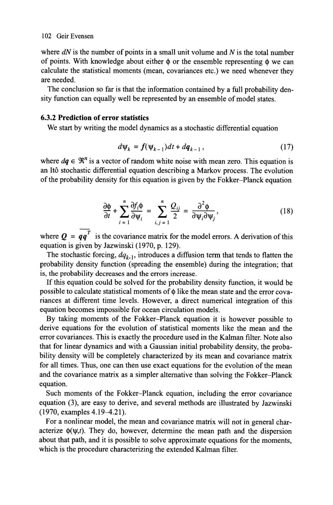
ofthe probability density for this equation is given by the Fokker-Planck equation
(18)
where Q = qqT is the covariance matrix for the model errors. A derivation ofthis
equation is given by Jazwinski (1970, p. 129).
The stochastic forcing, dqk-l' introduces a diffusion term that tends to flatten the
probability density function (spreading the ensemble) during the integration; that
is, the probability decreases and the errors increase.
If this equation could be solved for the probability density function, it would be
possible to calculate statistical moments of <1> like the mean state and the error covariances at different time levels. However, a direct numerical integration of this
equation becomes impossible for ocean circulation models.
By taking moments of the Fokker-Planck equation it is however possible to
derive equations for the evolution of statistical moments like the mean and the
error covariances. This is exactly the procedure used in the Kalman filter. Note also
that for linear dynamics and with a Gaussian initial probability density, the probability density will be completely characterized by its mean and covariance matrix
for alI times. Thus, one can then use exact equations for the evolution of the mean
and the covariance matrix as a simpler alternative than solving the Fokker-Planck
equation.
Such moments of the Fokker-Planck equation, inc1uding the error covariance
equation (3), are easy to derive, and several methods are ilIustrated by Jazwinski
(1970, examples 4.19-4.21).
For a nonlinear model, the mean and covariance matrix will not in general characterize (\jI,t). They do, however, determine the mean path and the dispersion
about that path, and it is possible to solve approximate equations for the moments,
which is the procedure characterizing the extended Kalman filter.
where dN is the number of points in a small unit volume and N is the total number
of points. With knowledge about either <1> or the ensemble representing <1> we can
calculate the statistical moments (mean, covariances etc.) we need whenever they
are needed.
The conc1usion so far is that the information contained by a full probability density function can equally well be represented by an ensemble of model states.
6.3.2 Prediction of error statistics
We start by writing the model dynamics as a stochastic differential equation
(17)
where dq E 9\n is a vector of random white noise with mean zero. This equation is
an !ta stochastic differential equation describing a Markov process. The evolution
ofthe probability density for this equation is given by the Fokker-Planck equation
(18)
where Q = qqT is the covariance matrix for the model errors. A derivation ofthis
equation is given by Jazwinski (1970, p. 129).
The stochastic forcing, dqk-l' introduces a diffusion term that tends to flatten the
probability density function (spreading the ensemble) during the integration; that
is, the probability decreases and the errors increase.
If this equation could be solved for the probability density function, it would be
possible to calculate statistical moments of <1> like the mean state and the error covariances at different time levels. However, a direct numerical integration of this
equation becomes impossible for ocean circulation models.
By taking moments of the Fokker-Planck equation it is however possible to
derive equations for the evolution of statistical moments like the mean and the
error covariances. This is exactly the procedure used in the Kalman filter. Note also
that for linear dynamics and with a Gaussian initial probability density, the probability density will be completely characterized by its mean and covariance matrix
for alI times. Thus, one can then use exact equations for the evolution of the mean
and the covariance matrix as a simpler alternative than solving the Fokker-Planck
equation.
Such moments of the Fokker-Planck equation, inc1uding the error covariance
equation (3), are easy to derive, and several methods are ilIustrated by Jazwinski
(1970, examples 4.19-4.21).
For a nonlinear model, the mean and covariance matrix will not in general characterize (\jI,t). They do, however, determine the mean path and the dispersion
about that path, and it is possible to solve approximate equations for the moments,
which is the procedure characterizing the extended Kalman filter.