

Sequential Data Assimilation for Nonlinear Dynamics: The Ensemble Kalman Filter
101
error covariance equation is proposed for the prediction of error statistics and
finally a consistent analysis scheme is presented.
6.3.1 Representation of error statistics
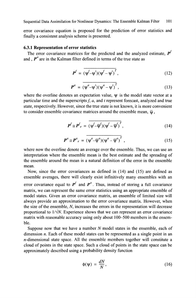
The error covariance matrices for the predicted and the analyzed estimate, pf
and , pa are in the Kalman filter defined in terms of the true state as
(12)
(13)
where the overline denotes an expectation value, '1' is the model state vector at a
particular time and the superscripts J, a, and t represent forecast, analyzed and true
state, respectively. However, since the true state is not known, it is more convenient
to consider ensemble covariance matrices around the ensemble mean, \ii,
(14)
a
a
a _a
a
_a T
p =p e = ('1' -'1' )('1' - '1') ,
(IS)
where now the overline denote an average over the ensemble. Thus, we can use an
interpretation where the ensemble mean is the best estimate and the spreading of
the ensemble around the mean is a natural definition of the error in the ensemble
mean.
Now, since the error covariances as defined in (14) and (1S) are defined as
ensemble averages, there will clearly exist infinitively many ensembles with an
error covariance equal to pf and pa . Thus, instead of storing a full covariance
matrix, we can represent the same error statistics using an appropriate ensemble of
model states. Given an error covariance matrix, an ensemble of limited size will
always provide an approximation to the error covariance matrix. However, when
the size of the ensemble, N, increases the errors in the representation will decrease
proportional to 1I-VN. Experience shows that we can represent an error covariance
matrix with reasonable accuracy using only about lO{}-SOO members in the ensembIe.
Suppose now that we have a number N model states in the ensemble, each of
dimension n. Each of these model states can be represented as a single point in an
n-dimensional state space. AH the ensemble members together will constitute a
cloud of points in the state space. Such a cloud of points in the state space can be
approximately described using a probability density function
dN
cI>('I') = li'
(16)
101
error covariance equation is proposed for the prediction of error statistics and
finally a consistent analysis scheme is presented.
6.3.1 Representation of error statistics
The error covariance matrices for the predicted and the analyzed estimate, pf
and , pa are in the Kalman filter defined in terms of the true state as
(12)
(13)
where the overline denotes an expectation value, '1' is the model state vector at a
particular time and the superscripts J, a, and t represent forecast, analyzed and true
state, respectively. However, since the true state is not known, it is more convenient
to consider ensemble covariance matrices around the ensemble mean, \ii,
(14)
a
a
a _a
a
_a T
p =p e = ('1' -'1' )('1' - '1') ,
(IS)
where now the overline denote an average over the ensemble. Thus, we can use an
interpretation where the ensemble mean is the best estimate and the spreading of
the ensemble around the mean is a natural definition of the error in the ensemble
mean.
Now, since the error covariances as defined in (14) and (1S) are defined as
ensemble averages, there will clearly exist infinitively many ensembles with an
error covariance equal to pf and pa . Thus, instead of storing a full covariance
matrix, we can represent the same error statistics using an appropriate ensemble of
model states. Given an error covariance matrix, an ensemble of limited size will
always provide an approximation to the error covariance matrix. However, when
the size of the ensemble, N, increases the errors in the representation will decrease
proportional to 1I-VN. Experience shows that we can represent an error covariance
matrix with reasonable accuracy using only about lO{}-SOO members in the ensembIe.
Suppose now that we have a number N model states in the ensemble, each of
dimension n. Each of these model states can be represented as a single point in an
n-dimensional state space. AH the ensemble members together will constitute a
cloud of points in the state space. Such a cloud of points in the state space can be
approximately described using a probability density function
dN
cI>('I') = li'
(16)