

Sequential Data Assimilation for Nonlinear Dynamics: The Ensemble Kalman Filter
99
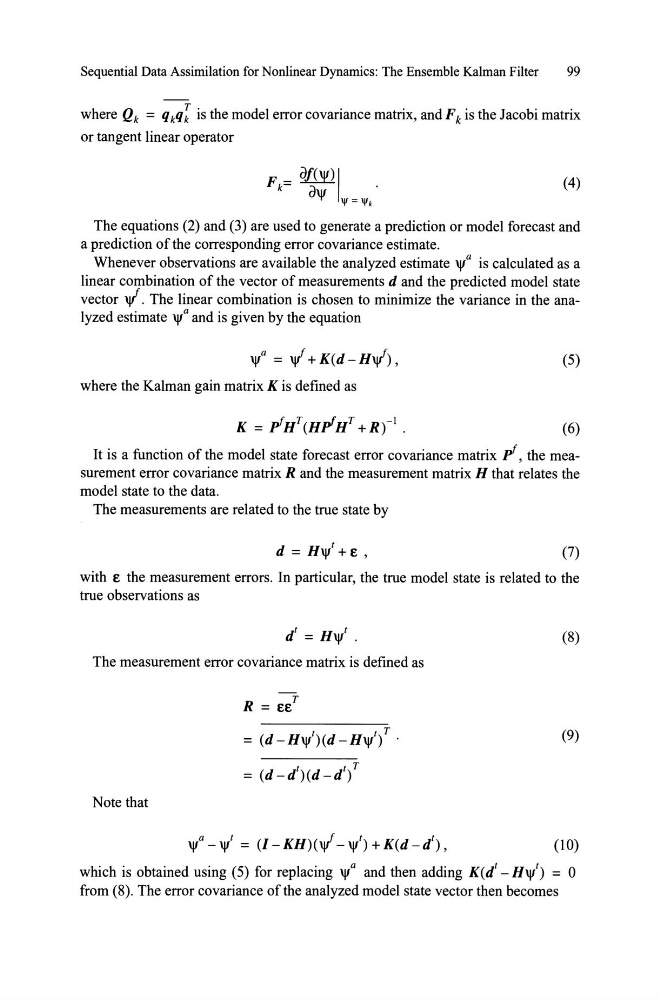
where Qk = q kq[ is the model error covariance matrix, and F k is the Jacobi matrix
or tangent linear operator
F-~I k- ali(
'f'
IJI = IJIk
(4)
The equations (2) and (3) are used to generate a prediction or model forecast and
a prediction of the corresponding error covariance estimate.
Whenever observations are available the analyzed estimate \jIa is calculated as a
linear combination of the vector of measurements d and the predicted model state
vector ~. The linear combination is chosen to minimize the variance in the analyzed estimate \jIa and is given by the equation
\jIa = ~+K(d-H~),
(5)
where the Kalman gain matrix K is defined as
(6)
It is a function of the model state forecast error covariance matrix pf, the measurement error covariance matrix R and the measurement matrix H that relates the
model state to the data.
The measurements are related to the true state by
(7)
with E the measurement errors. In particular, the true model state is related to the
true observations as
d t = H\jIt .
(8)
The measurement error covariance matrix is defined as
t
t T
= (d-H\jI)(d-H\jI) .
(9)
= (d _dt)(d _d t {
Note that
(10)
which is obtained using (5) for replacing \jIa and then adding K(i - H\jIt) = O
from (8). The error covariance ofthe analyzed model state vector then becomes
99
where Qk = q kq[ is the model error covariance matrix, and F k is the Jacobi matrix
or tangent linear operator
F-~I k- ali(
'f'
IJI = IJIk
(4)
The equations (2) and (3) are used to generate a prediction or model forecast and
a prediction of the corresponding error covariance estimate.
Whenever observations are available the analyzed estimate \jIa is calculated as a
linear combination of the vector of measurements d and the predicted model state
vector ~. The linear combination is chosen to minimize the variance in the analyzed estimate \jIa and is given by the equation
\jIa = ~+K(d-H~),
(5)
where the Kalman gain matrix K is defined as
(6)
It is a function of the model state forecast error covariance matrix pf, the measurement error covariance matrix R and the measurement matrix H that relates the
model state to the data.
The measurements are related to the true state by
(7)
with E the measurement errors. In particular, the true model state is related to the
true observations as
d t = H\jIt .
(8)
The measurement error covariance matrix is defined as
t
t T
= (d-H\jI)(d-H\jI) .
(9)
= (d _dt)(d _d t {
Note that
(10)
which is obtained using (5) for replacing \jIa and then adding K(i - H\jIt) = O
from (8). The error covariance ofthe analyzed model state vector then becomes