

92 Andrew C. Lorenc
C o = GnnGn_1oo. nG 2 nG 1
CI=GnnGn_loo.nG2nGI
C 2 = GnnGn_1oo. nG2nGI
C"
= Gn (î Gnloo. n G2 (î GI
2 -1
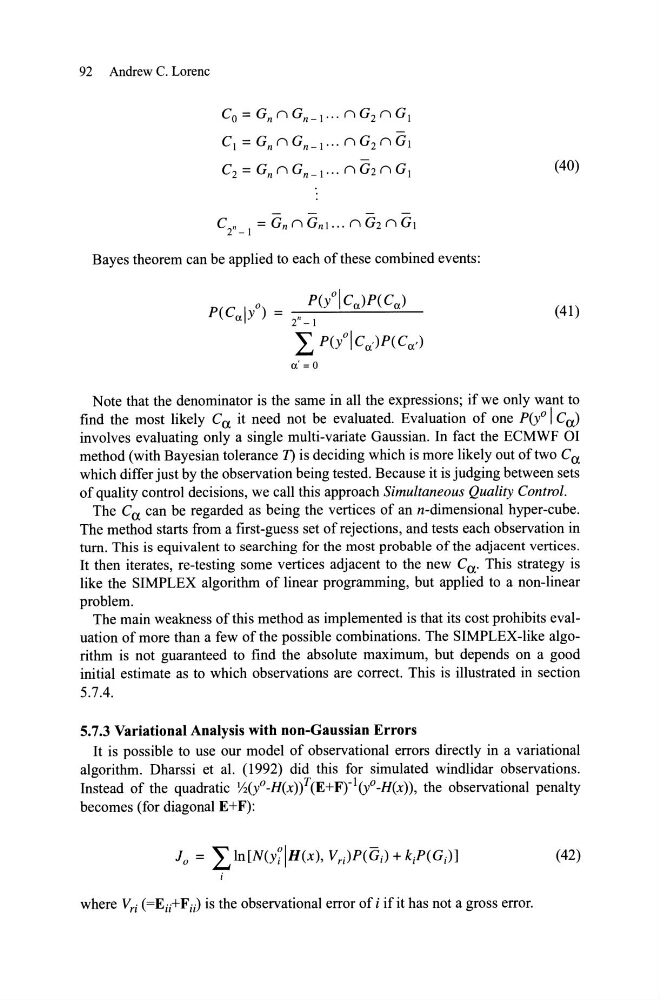
Bayes theorem can be applied to each ofthese combined events:
2" - 1
L p(lICa,)p(C a ,)
a' = O
(40)
(41)
Note that the denominator is the same in all the expressions; ifwe only want to
find the most likely Ca it need not be evaluated. Evaluation of one P(f I Ca)
involves evaluating only a single multi-variate Gaussian. In fact the ECMWF OI
method (with Bayesian tolerance 1) is deciding which is more likely out oftwo Ca
which differ just by the observation being tested. Because it is judging between sets
of quality control decisions, we call this approach Simultaneous Quality Control.
The Ca can be regarded as being the vertices of an n-dimensional hyper-cube.
The method starts from a first-guess set of rejections, and tests each observation in
turn. This is equivalent to searching for the most probable of the adjacent vertices.
It then iterates, re-testing some vertices adjacent to the new Ca' This strategy is
like the SIMPLEX algorithm of linear programming, but applied to a non-linear
problem.
The main weakness of this method as implemented is that its cost prohibits evaluation of more than a few of the possible combinations. The SIMPLEX-like algorithm is not guaranteed to find the absolute maximum, but depends on a good
initial estimate as to which observations are correct. This is illustrated in section
5.7.4.
5.7.3 Variational Analysis with non-Gaussian Errors
It is possible to use our model of observational errors directly in a variational
algorithm. Dharssi et al. (1992) did this for simulated windlidar observations.
Instead of the quadratic Y2(y°-H(x))T(E+Fr 1 (y°-H(x)), the observational penalty
becomes (for diagonal E+F):
(42)
where V rÎ (= Eii+ F ii) is the observational error of i if it has not a gross error.
C o = GnnGn_1oo. nG 2 nG 1
CI=GnnGn_loo.nG2nGI
C 2 = GnnGn_1oo. nG2nGI
C"
= Gn (î Gnloo. n G2 (î GI
2 -1
Bayes theorem can be applied to each ofthese combined events:
2" - 1
L p(lICa,)p(C a ,)
a' = O
(40)
(41)
Note that the denominator is the same in all the expressions; ifwe only want to
find the most likely Ca it need not be evaluated. Evaluation of one P(f I Ca)
involves evaluating only a single multi-variate Gaussian. In fact the ECMWF OI
method (with Bayesian tolerance 1) is deciding which is more likely out oftwo Ca
which differ just by the observation being tested. Because it is judging between sets
of quality control decisions, we call this approach Simultaneous Quality Control.
The Ca can be regarded as being the vertices of an n-dimensional hyper-cube.
The method starts from a first-guess set of rejections, and tests each observation in
turn. This is equivalent to searching for the most probable of the adjacent vertices.
It then iterates, re-testing some vertices adjacent to the new Ca' This strategy is
like the SIMPLEX algorithm of linear programming, but applied to a non-linear
problem.
The main weakness of this method as implemented is that its cost prohibits evaluation of more than a few of the possible combinations. The SIMPLEX-like algorithm is not guaranteed to find the absolute maximum, but depends on a good
initial estimate as to which observations are correct. This is illustrated in section
5.7.4.
5.7.3 Variational Analysis with non-Gaussian Errors
It is possible to use our model of observational errors directly in a variational
algorithm. Dharssi et al. (1992) did this for simulated windlidar observations.
Instead of the quadratic Y2(y°-H(x))T(E+Fr 1 (y°-H(x)), the observational penalty
becomes (for diagonal E+F):
(42)
where V rÎ (= Eii+ F ii) is the observational error of i if it has not a gross error.