

Atmospheric Data Assimilation and Quality Control
77
If our observation directly measures the variable x, with observational error variance \1', then the probability of observed value yO, given the true value is x, can
also be modelled by a Gaussian pdf:
We can get p(y0) by integrating over all x:
--- p(y") = fp(/lx)p(x)dX
For Gaussians (6) and (7) this gives:
p(/) = N(/Ii, V' + v")
Substituting in (5) gives:
where
a
o
b
~=L+~
v" v" v"
1
1
1
-=-+v" V' v"
(7)
(8)
(9)
(lO)
(II)
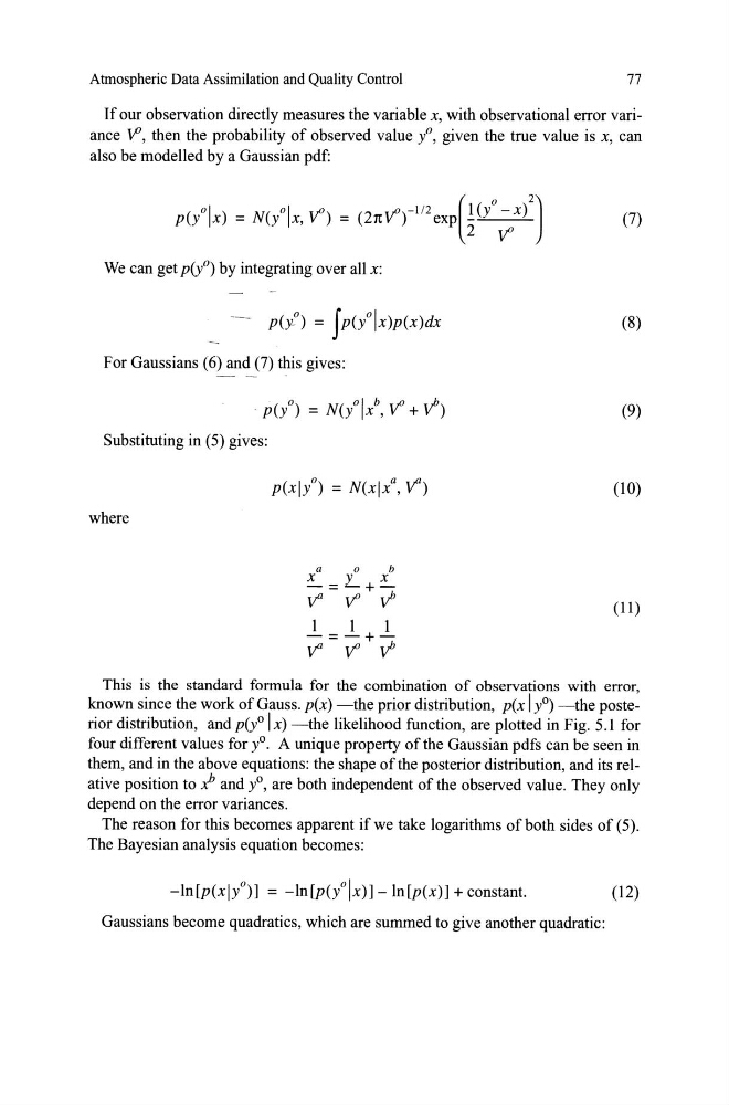
This is the standard formula for the combination of observations with error,
known since the work of Gauss. p(x) -the prior distribution, p(x I yO) -the posterior distribution, and p(y°l x) -the likelihood function, are plotted in Fig. 5.1 for
four different values for yO. A unique property ofthe Gaussian pdfs can be seen in
them, and in the above equations: the shape of the posterior distribution, and its relative position to jJ and yO, are both independent of the observed value. They only
depend on the error variances.
The reason for this becomes apparent ifwe take logarithms ofboth sides of (5).
The Bayesian analysis equation becomes:
-ln[p(xi/)] = -ln[p(/Ix)] -ln[p(x)] + constant.
(12)
Gaussians become quadratics, which are summed to give another quadratic:
77
If our observation directly measures the variable x, with observational error variance \1', then the probability of observed value yO, given the true value is x, can
also be modelled by a Gaussian pdf:
We can get p(y0) by integrating over all x:
--- p(y") = fp(/lx)p(x)dX
For Gaussians (6) and (7) this gives:
p(/) = N(/Ii, V' + v")
Substituting in (5) gives:
where
a
o
b
~=L+~
v" v" v"
1
1
1
-=-+v" V' v"
(7)
(8)
(9)
(lO)
(II)
This is the standard formula for the combination of observations with error,
known since the work of Gauss. p(x) -the prior distribution, p(x I yO) -the posterior distribution, and p(y°l x) -the likelihood function, are plotted in Fig. 5.1 for
four different values for yO. A unique property ofthe Gaussian pdfs can be seen in
them, and in the above equations: the shape of the posterior distribution, and its relative position to jJ and yO, are both independent of the observed value. They only
depend on the error variances.
The reason for this becomes apparent ifwe take logarithms ofboth sides of (5).
The Bayesian analysis equation becomes:
-ln[p(xi/)] = -ln[p(/Ix)] -ln[p(x)] + constant.
(12)
Gaussians become quadratics, which are summed to give another quadratic: