

78 Andrew C. Lorenc
/ '
/
'\
I \
\
\
\
\
\
\
\
/ '
/
/ '
/
\
,
\
\
\
\
\
\
\
\ ,
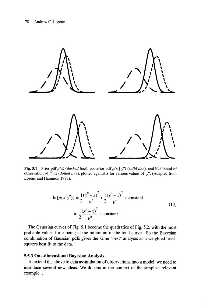
Fig.5.1 Prior pdf p(x) (dashed line), posterior pdf p(x I yo) (solid line), and likelihood of
observation p(yOI x) (dotted line), plotted against x for various values of yO. (Adapted from
Lorenc and Hammon 1988).
b
2
° 2
°
1 (x - x)
1 (y - x)
-ln[p(xly )] = -
+ -
+ constant
2yh
2v"
a
2
= ! (X - X) + constant.
2 v"
(13)
The Gaussian curves of Fig. 5.1 become the quadratics of Fig. 5.2, with the most
probable values for x being at the minimum of the total curve. So the Bayesian
combination of Gaussian pdfs gives the same "best" analysis as a weighted leastsquares best fit to the data.
5.5.3 One-dimensional Bayesian Analysis
To extend the above to data assimilation of observations into a model, we need to
introduce several new ideas. We do this in the context of the simplest relevant
example: .
/ '
/
'\
I \
\
\
\
\
\
\
\
/ '
/
/ '
/
\
,
\
\
\
\
\
\
\
\ ,
Fig.5.1 Prior pdf p(x) (dashed line), posterior pdf p(x I yo) (solid line), and likelihood of
observation p(yOI x) (dotted line), plotted against x for various values of yO. (Adapted from
Lorenc and Hammon 1988).
b
2
° 2
°
1 (x - x)
1 (y - x)
-ln[p(xly )] = -
+ -
+ constant
2yh
2v"
a
2
= ! (X - X) + constant.
2 v"
(13)
The Gaussian curves of Fig. 5.1 become the quadratics of Fig. 5.2, with the most
probable values for x being at the minimum of the total curve. So the Bayesian
combination of Gaussian pdfs gives the same "best" analysis as a weighted leastsquares best fit to the data.
5.5.3 One-dimensional Bayesian Analysis
To extend the above to data assimilation of observations into a model, we need to
introduce several new ideas. We do this in the context of the simplest relevant
example: .