76 Andrew C. Lorenc
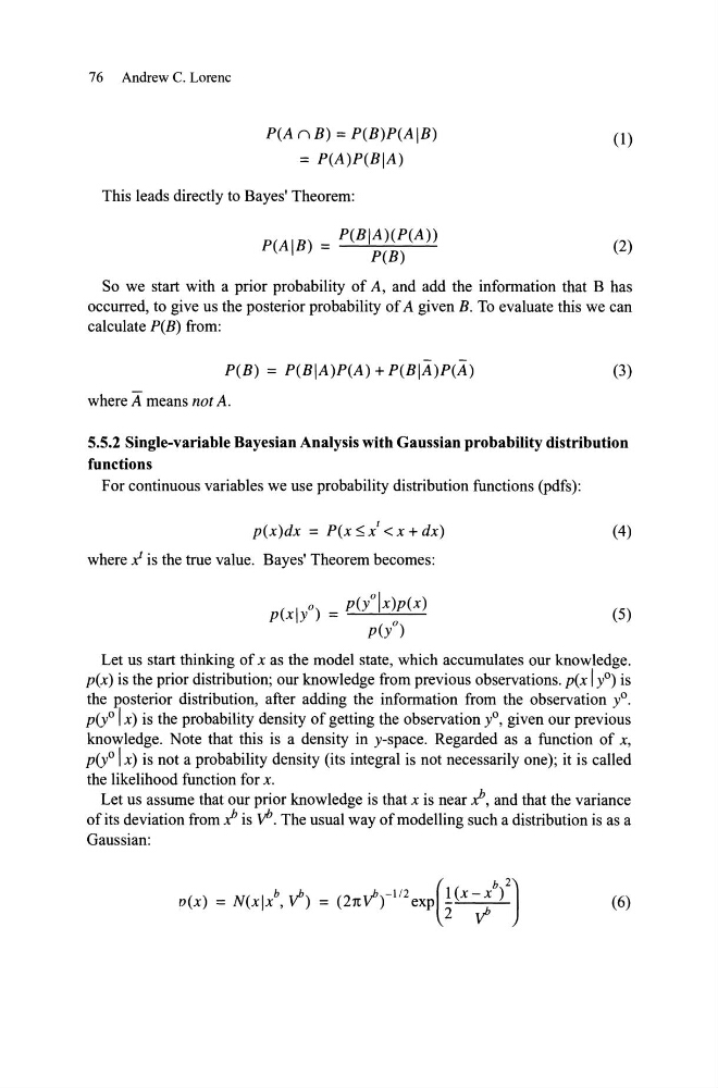
P(A n B) = P(B)P(AIB)
= P(A)P(BIA)
This leads direct1y to Bayes' Theorem:
P(AIB) = P(BIA)(P(A»
P(B)
(1)
(2)
So we start with a prior probability of A, and add the information that B has
occurred, to give us the posterior probability of A given B. To evaluate this we can
calculate P(B) from:
P(B) = P(BIA)P(A) + P(BIA)P(A)
where A means not A.
(3)
5.5.2 Single-variable Bayesian Analysis with Gaussian probability distribution
functions
For continuous variables we use probability distribution functions (Pdfs):
p(x)dx = P(x~/ where x t is the true value. Bayes' Theorem becomes:
(4)
(5)
Let us start thinking of x as the model state, which accumulates our knowledge.
p(x) is the prior distribution; our knowledge from previous observations. p(x I yO) is
the posterior distribution, after adding the information from the observation yO.
p(y0 Ix) is the probability density of getting the observation yO, given our previous
knowledge. Note that this is a density in y-space. Regarded as a function of x,
p(y0 Ix) is not a probability density (its integral is not necessarily one); it is called
the likelihood function for x.
Let us assume that our prior knowledge is that x is near Y!, and that the variance
of its deviation from Y! is vi'. The usual way of modelling such a distribution is as a
Gaussian:
b
-112
1 x-x
(
b 2)
o(x) = N(xlx , V') = (21tV') exp 2: ( V')
(6)