

238
Theory of the Ventilated Thermocline
layer at its most northern extent and, to maintain the static stability of the
system, is always less than the density of the layer beneath it. Thus, at () = () 3
the mixed layer density is p 2 and decreases smoothly southward to become p 1
at () = e2. Both the mixed layer depth and density are taken to be functions
only of latitude for simplicity, as are the outcrop lines.
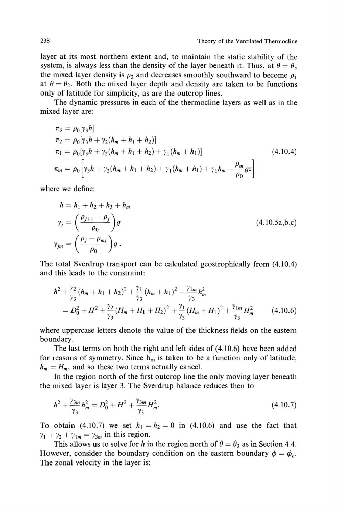
The dynamic pressures in each of the thermocline layers as well as in the
mixed layer are:
1t3 = Po[Y3h]
1t2 = Po[Y3h + Y2(hm + h, + h2)]
1t1 = Po[Y3h + Y2(hm + h, + h2) + y, (hm +hi)]
(4.10.4)
1tm =Po [y3h + Y2(hm + h1 + h2) + Y! (hm +hi)+ Y!hm- ~: gz]
where we define:
Y· =(PH!- PJ)g
1
Po
(4.10.5a,b,c)
Yjm = (Pj ~:mj )g.
The total Sverdrup transport can be calculated geostrophically from (4.10.4)
and this leads to the constraint:
h2 + Y2 (hm + h! + h2)2 + 1J. (hm + h!)2 + Y!m h~
h
h
h
= JYo + H2 + Y2 (Hm + H, + H2)2 + Y! (Hm + H,)2 + Y!m H;,
h
h
h
(4.10.6)
where uppercase letters denote the value of the thickness fields on the eastern
boundary.
The last terms on both the right and left sides of(4.10.6) have been added
for reasons of symmetry. Since hm is taken to be a function only of latitude,
hm = Hm, and so these two terms actually cancel.
In the region north of the first outcrop line the only moving layer beneath
the mixed layer is layer 3. The Sverdrup balance reduces then to:
(4.10.7)
To obtain (4.10.7) we set h1 = h2 = 0 in (4.10.6) and use the fact that
Y! + Y2 + Y!m = y3m in this region.
This allows us to solve for h in the region north of() = ()3 as in Section 4.4.
However, consider the boundary condition on the eastern boundary ¢ = ¢e·
The zonal velocity in the layer is:
Theory of the Ventilated Thermocline
layer at its most northern extent and, to maintain the static stability of the
system, is always less than the density of the layer beneath it. Thus, at () = () 3
the mixed layer density is p 2 and decreases smoothly southward to become p 1
at () = e2. Both the mixed layer depth and density are taken to be functions
only of latitude for simplicity, as are the outcrop lines.
The dynamic pressures in each of the thermocline layers as well as in the
mixed layer are:
1t3 = Po[Y3h]
1t2 = Po[Y3h + Y2(hm + h, + h2)]
1t1 = Po[Y3h + Y2(hm + h, + h2) + y, (hm +hi)]
(4.10.4)
1tm =Po [y3h + Y2(hm + h1 + h2) + Y! (hm +hi)+ Y!hm- ~: gz]
where we define:
Y· =(PH!- PJ)g
1
Po
(4.10.5a,b,c)
Yjm = (Pj ~:mj )g.
The total Sverdrup transport can be calculated geostrophically from (4.10.4)
and this leads to the constraint:
h2 + Y2 (hm + h! + h2)2 + 1J. (hm + h!)2 + Y!m h~
h
h
h
= JYo + H2 + Y2 (Hm + H, + H2)2 + Y! (Hm + H,)2 + Y!m H;,
h
h
h
(4.10.6)
where uppercase letters denote the value of the thickness fields on the eastern
boundary.
The last terms on both the right and left sides of(4.10.6) have been added
for reasons of symmetry. Since hm is taken to be a function only of latitude,
hm = Hm, and so these two terms actually cancel.
In the region north of the first outcrop line the only moving layer beneath
the mixed layer is layer 3. The Sverdrup balance reduces then to:
(4.10.7)
To obtain (4.10.7) we set h1 = h2 = 0 in (4.10.6) and use the fact that
Y! + Y2 + Y!m = y3m in this region.
This allows us to solve for h in the region north of() = ()3 as in Section 4.4.
However, consider the boundary condition on the eastern boundary ¢ = ¢e·
The zonal velocity in the layer is: