

Effect of Finite Mixed Layer Depth
237
-----------------t----z3
P3
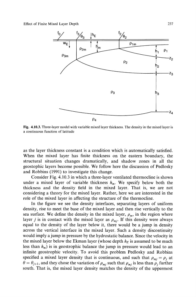
Fig. 4.10.3. Three-layer model with variable mixed layer thickness. The density in the mixed layer is
a continuous function of latitude
as the layer thickness constant is a condition which is automatically satisfied.
When the mixed layer has finite thickness on the eastern boundary, the
structural situation changes dramatically, and shadow zones in all the
geostophic layers become possible. We follow here the discussion of Pedlosky
and Robbins (1991) to investigate this change.
Consider Fig. 4.10.3 in which a three-layer ventilated thermocline is shown
under a mixed layer of variable thickness hm. We specify below both the
thickness and the density field in the mixed layer. That is, we are not
considering a theory for the mixed layer. Rather, here we are interested in the
role of the mixed layer in affecting the structure of the thermocline.
In the figure we see the density interfaces, separating layers of uniform
density, rise to meet the base of the mixed layer and then rise vertically to the
sea surface. We define the density in the mixed layer, Pm• in the region where
layer j is in contact with the mixed layer as PmJ· If this density were always
equal to the density of the layer below it, there would be a jump in density
across the vertical interface in the mixed layer. Such a density discontinuity
would imply a jump in pressure by the hydrostatic balance. Since the velocity in
the mixed layer below the Ekman layer (whose depth hE is assumed to be much
less than hm) is in geostrophic balance the jump in pressure would lead to an
infinite geostrophic velocity. To avoid this problem Pedlosky and Robbins
specified a mixed layer density that is continuous, and such that PmJ = p 1 at
(} = (}J+I, and they chose the variation of PmJ such that PmJ is less than p 1 further
south. That is, the mixed layer density matches the density of the uppermost
237
-----------------t----z3
P3
Fig. 4.10.3. Three-layer model with variable mixed layer thickness. The density in the mixed layer is
a continuous function of latitude
as the layer thickness constant is a condition which is automatically satisfied.
When the mixed layer has finite thickness on the eastern boundary, the
structural situation changes dramatically, and shadow zones in all the
geostophic layers become possible. We follow here the discussion of Pedlosky
and Robbins (1991) to investigate this change.
Consider Fig. 4.10.3 in which a three-layer ventilated thermocline is shown
under a mixed layer of variable thickness hm. We specify below both the
thickness and the density field in the mixed layer. That is, we are not
considering a theory for the mixed layer. Rather, here we are interested in the
role of the mixed layer in affecting the structure of the thermocline.
In the figure we see the density interfaces, separating layers of uniform
density, rise to meet the base of the mixed layer and then rise vertically to the
sea surface. We define the density in the mixed layer, Pm• in the region where
layer j is in contact with the mixed layer as PmJ· If this density were always
equal to the density of the layer below it, there would be a jump in density
across the vertical interface in the mixed layer. Such a density discontinuity
would imply a jump in pressure by the hydrostatic balance. Since the velocity in
the mixed layer below the Ekman layer (whose depth hE is assumed to be much
less than hm) is in geostrophic balance the jump in pressure would lead to an
infinite geostrophic velocity. To avoid this problem Pedlosky and Robbins
specified a mixed layer density that is continuous, and such that PmJ = p 1 at
(} = (}J+I, and they chose the variation of PmJ such that PmJ is less than p 1 further
south. That is, the mixed layer density matches the density of the uppermost